#======================================================
# Use of numpy

import numpy as np

def relu(x):
    """ReLU activation function."""
    return np.maximum(0, x)

# 1. Setup Data with Teacher Data
# N: Total samples, D_in: Input dimension
# H1, H2: Hidden dimensions, D_out: Output dimension
N, D_in, H1, H2, D_out = 500, 10, 100, 50, 1

# Generate synthetic input data
np.random.seed(42)
x_all = np.random.randn(N, D_in)

# Generate "Teacher Data" (Ground Truth)
# Let's define a non-linear relationship: y = sum(x^2) + noise
y_all = np.sum(x_all**2, axis=1, keepdims=True) + 0.1 * np.random.randn(N, 1)

# Split into Train and Test
split_idx = int(N * 0.8)
x_train, x_test = x_all[:split_idx], x_all[split_idx:]
y_train, y_test = y_all[:split_idx], y_all[split_idx:]

print(f"Data Shapes: Train x={x_train.shape}, y={y_train.shape} | Test x={x_test.shape}, y={y_test.shape}")

# 2. Initialize Weights
w1 = np.random.randn(D_in, H1) * 0.01
w2 = np.random.randn(H1, H2) * 0.01
w3 = np.random.randn(H2, D_out) * 0.01

learning_rate = 1e-4 # Slightly larger LR often helps with small init
print(f"Training NumPy 3-Layer NN for 1000 steps...")

for t in range(1001):
    # --- Forward Pass (Training) ---
    # Layer 1
    h1 = x_train.dot(w1)
    h1_relu = relu(h1)

    # Layer 2
    h2 = h1_relu.dot(w2)
    h2_relu = relu(h2)

    # Layer 3 (Output)
    y_pred = h2_relu.dot(w3)

    # Compute Loss (MSE)
    loss = np.mean(np.square(y_pred - y_train))
    if t % 100 == 0:
        print(f"Step {t}: Train Loss = {loss:.4f}")

    # --- Backward Pass (Manual Gradients) ---
    # dLoss/dy_pred = 2 * (y_pred - y) / N (because we used mean)
    grad_y_pred = 2.0 * (y_pred - y_train) / x_train.shape[0]

    # Backprop through Layer 3
    grad_w3 = h2_relu.T.dot(grad_y_pred)
    grad_h2_relu = grad_y_pred.dot(w3.T)

    # Backprop through ReLU 2
    grad_h2 = grad_h2_relu.copy()
    grad_h2[h2 < 0] = 0

    # Backprop through Layer 2
    grad_w2 = h1_relu.T.dot(grad_h2)
    grad_h1_relu = grad_h2.dot(w2.T)

    # Backprop through ReLU 1
    grad_h1 = grad_h1_relu.copy()
    grad_h1[h1 < 0] = 0

    # Backprop through Layer 1
    grad_w1 = x_train.T.dot(grad_h1)

    # --- Update Weights ---
    w1 -= learning_rate * grad_w1
    w2 -= learning_rate * grad_w2
    w3 -= learning_rate * grad_w3

print("Training Complete.")

# 3. Model Evaluation
print("\n--- Model Evaluation ---")
# Forward pass on Test Data
h1_test = x_test.dot(w1)
h1_relu_test = relu(h1_test)

h2_test = h1_relu_test.dot(w2)
h2_relu_test = relu(h2_test)

y_pred_test = h2_relu_test.dot(w3)

# Compute Test Loss
test_loss = np.mean(np.square(y_pred_test - y_test))
print(f"Test Loss: {test_loss:.4f}")

# Compare first 5 predictions
print("\nFirst 5 Predictions vs Ground Truth:")
for i in range(5):
    print(f"Pred: {y_pred_test[i][0]:.4f} | True: {y_test[i][0]:.4f}")

#=================================================================
# Use of torch
import torch
import time

start_time = time.time()
import torch.nn as nn
import torch.optim as optim

# 1. Setup Data with Teacher Data
# N: Total samples, D_in: Input dimension
# H1, H2: Hidden dimensions, D_out: Output dimension
N, D_in, H1, H2, D_out = 500, 10, 100, 50, 1

# Generate synthetic input data
torch.manual_seed(42)
x_all = torch.randn(N, D_in)

# Generate "Teacher Data" (Ground Truth)
# Relationship: y = sum(x^2) + noise
y_all = torch.sum(x_all**2, dim=1, keepdim=True) + 0.1 * torch.randn(N, 1)

# Split into Train and Test
split_idx = int(N * 0.8)
x_train, x_test = x_all[:split_idx], x_all[split_idx:]
y_train, y_test = y_all[:split_idx], y_all[split_idx:]

print(f"Data Shapes: Train x={x_train.shape}, y={y_train.shape} | Test x={x_test.shape}, y={y_test.shape}")

# 2. Define Model
model = nn.Sequential(
    nn.Linear(D_in, H1),
    nn.ReLU(),
    nn.Linear(H1, H2),
    nn.ReLU(),
    nn.Linear(H2, D_out)
)

# Loss and Optimizer
loss_fn = nn.MSELoss()
optimizer = optim.Adam(model.parameters(), lr=1e-3)

print("Training PyTorch 3-Layer NN for 1000 steps...")

for t in range(1001):
    # --- Forward Pass ---
    y_pred = model(x_train)

    # --- Compute Loss ---
    loss = loss_fn(y_pred, y_train)

    if t % 100 == 0:
        print(f"Step {t}: Train Loss = {loss.item():.4f}")

    # --- Backward Pass ---
    optimizer.zero_grad()
    loss.backward()
    optimizer.step()

print("Training Complete.")

# 3. Model Evaluation
print("\n--- Model Evaluation ---")
model.eval() # Set model to evaluation mode
with torch.no_grad(): # Disable gradient calculation
    y_pred_test = model(x_test)
    test_loss = loss_fn(y_pred_test, y_test)
    print(f"Test Loss: {test_loss.item():.4f}")

    # Compare first 5 predictions
    print("\nFirst 5 Predictions vs Ground Truth:")
    for i in range(5):
        print(f"Pred: {y_pred_test[i].item():.4f} | True: {y_test[i].item():.4f}")

end_time = time.time()
print(f"\nTotal Execution Time: {end_time - start_time:.4f} seconds")
Author: Alumi-Lab
Three Layer NNet execution times (CPU vs GPU)
Gemini 3 Proがまとめた、三層ニューラルネットワークのプロジェクトの説明です。
=========================
# プロジェクト概要: PyTorch ニューラルネットワーク (CUDA対応)
## 1. ユーザー(浦田)からの要望と目的
*   **目的:** `three_layer_nn_pytorch.py` を修正し、NVIDIA GPU (CUDA) 処理をサポートする新しいスクリプト `three_layer_nn_pytorch_cuda.py` を作成する。
*   **要望 1:** GPU処理用のデバイスを定義し、データとモデルをそのデバイスに移動するための必要な修正を行う。
*   **要望 2:** 比較のために、元のCPU用スクリプト (`three_layer_nn_pytorch.py`) も実行する。
*   **要望 3:** `time` モジュールをインポートし、両方のスクリプトの実行時間を計測して出力する。
*   **要望 4:** ベンチマークを実行し、両方のスクリプトの実行時間を比較する。
*   **最終要望:** これまでの作業、回答、要望をすべて1つのファイルに保存する。
## 2. コード実装
### A. CUDA 実装 (`three_layer_nn_pytorch_cuda.py`)
このスクリプトはCUDAの利用可能性を確認し、モデルとテンソルをGPUに移動させ、実行時間を計測します。
```python
import torch
import time
start_time = time.time()
import torch.nn as nn
import torch.optim as optim
# デバイスの定義
device = torch.device("cuda" if torch.cuda.is_available() else "cpu")
print(f"Using device: {device}")
# 1. データのセットアップ (教師データ付き)
# N: サンプル総数, D_in: 入力次元
# H1, H2: 隠れ層の次元, D_out: 出力次元
N, D_in, H1, H2, D_out = 500, 10, 100, 50, 1
# 合成入力データの生成
torch.manual_seed(42)
x_all = torch.randn(N, D_in)
# "教師データ" (正解データ) の生成
# 関係式: y = sum(x^2) + noise
y_all = torch.sum(x_all**2, dim=1, keepdim=True) + 0.1 * torch.randn(N, 1)
# 学習用とテスト用に分割
split_idx = int(N * 0.😎
x_train, x_test = x_all[:split_idx], x_all[split_idx:]
y_train, y_test = y_all[:split_idx], y_all[split_idx:]
# データをデバイスへ移動
x_train = x_train.to(device)
y_train = y_train.to(device)
x_test = x_test.to(device)
y_test = y_test.to(device)
print(f"Data Shapes: Train x={x_train.shape}, y={y_train.shape} | Test x={x_test.shape}, y={y_test.shape}")
# 2. モデルの定義
model = nn.Sequential(
    nn.Linear(D_in, H1),
    nn.ReLU(),
    nn.Linear(H1, H2),
    nn.ReLU(),
    nn.Linear(H2, D_out)
)
model.to(device)
# 損失関数とオプティマイザ
loss_fn = nn.MSELoss()
optimizer = optim.Adam(model.parameters(), lr=1e-3)
print("Training PyTorch 3-Layer NN for 1000 steps...")
for t in range(1001):
    # --- 順伝播 (Forward Pass) ---
    y_pred = model(x_train)
    # --- 損失の計算 ---
    loss = loss_fn(y_pred, y_train)
    if t % 100 == 0:
        print(f"Step {t}: Train Loss = {loss.item():.4f}")
    # --- 逆伝播 (Backward Pass) ---
    optimizer.zero_grad()
    loss.backward()
    optimizer.step()
print("Training Complete.")
# 3. モデルの評価
print("\n--- Model Evaluation ---")
model.eval() # モデルを評価モードに設定
with torch.no_grad(): # 勾配計算を無効化
    y_pred_test = model(x_test)
    test_loss = loss_fn(y_pred_test, y_test)
    print(f"Test Loss: {test_loss.item():.4f}")
    # 最初の5つの予測結果を正解と比較
    print("\nFirst 5 Predictions vs Ground Truth:")
    for i in range(5):
        print(f"Pred: {y_pred_test[i].item():.4f} | True: {y_test[i].item():.4f}")
end_time = time.time()
print(f"\nTotal Execution Time: {end_time - start_time:.4f} seconds")
```
### B. CPU 実装 (`three_layer_nn_pytorch.py`)
元のスクリプトに実行時間の計測機能を追加したものです。
```python
import torch
import time
start_time = time.time()
import torch.nn as nn
import torch.optim as optim
# 1. データのセットアップ (教師データ付き)
# N: サンプル総数, D_in: 入力次元
# H1, H2: 隠れ層の次元, D_out: 出力次元
N, D_in, H1, H2, D_out = 500, 10, 100, 50, 1
# 合成入力データの生成
torch.manual_seed(42)
x_all = torch.randn(N, D_in)
# "教師データ" (正解データ) の生成
# 関係式: y = sum(x^2) + noise
y_all = torch.sum(x_all**2, dim=1, keepdim=True) + 0.1 * torch.randn(N, 1)
# 学習用とテスト用に分割
split_idx = int(N * 0.😎
x_train, x_test = x_all[:split_idx], x_all[split_idx:]
y_train, y_test = y_all[:split_idx], y_all[split_idx:]
print(f"Data Shapes: Train x={x_train.shape}, y={y_train.shape} | Test x={x_test.shape}, y={y_test.shape}")
# 2. モデルの定義
model = nn.Sequential(
    nn.Linear(D_in, H1),
    nn.ReLU(),
    nn.Linear(H1, H2),
    nn.ReLU(),
    nn.Linear(H2, D_out)
)
# 損失関数とオプティマイザ
loss_fn = nn.MSELoss()
optimizer = optim.Adam(model.parameters(), lr=1e-3)
print("Training PyTorch 3-Layer NN for 1000 steps...")
for t in range(1001):
    # --- 順伝播 (Forward Pass) ---
    y_pred = model(x_train)
    # --- 損失の計算 ---
    loss = loss_fn(y_pred, y_train)
    if t % 100 == 0:
        print(f"Step {t}: Train Loss = {loss.item():.4f}")
    # --- 逆伝播 (Backward Pass) ---
    optimizer.zero_grad()
    loss.backward()
    optimizer.step()
print("Training Complete.")
# 3. モデルの評価
print("\n--- Model Evaluation ---")
model.eval() # モデルを評価モードに設定
with torch.no_grad(): # 勾配計算を無効化
    y_pred_test = model(x_test)
    test_loss = loss_fn(y_pred_test, y_test)
    print(f"Test Loss: {test_loss.item():.4f}")
    # 最初の5つの予測結果を正解と比較
    print("\nFirst 5 Predictions vs Ground Truth:")
    for i in range(5):
        print(f"Pred: {y_pred_test[i].item():.4f} | True: {y_test[i].item():.4f}")
end_time = time.time()
print(f"\nTotal Execution Time: {end_time - start_time:.4f} seconds")
```
## 3. ベンチマーク結果
両方のスクリプトを実行して得られた結果は以下の通りです。
```text
Running CPU Benchmark...
Data Shapes: Train x=torch.Size([400, 10]), y=torch.Size([400, 1]) | Test x=torch.Size([100, 10]), y=torch.Size([100, 1])
Training PyTorch 3-Layer NN for 1000 steps...
Step 0: Train Loss = 116.9025
Step 100: Train Loss = 5.9574
Step 200: Train Loss = 4.2802
Step 300: Train Loss = 3.1939
Step 400: Train Loss = 2.3619
Step 500: Train Loss = 1.6937
Step 600: Train Loss = 1.0309
Step 700: Train Loss = 0.3991
Step 800: Train Loss = 0.1677
Step 900: Train Loss = 0.0998
Step 1000: Train Loss = 0.0627
Training Complete.
--- Model Evaluation ---
Test Loss: 2.1775
First 5 Predictions vs Ground Truth:
Pred: 13.2606 | True: 15.5540
Pred: 12.4809 | True: 11.7322
Pred: 10.6773 | True: 10.5252
Pred: 7.9598 | True: 8.2041
Pred: 12.2528 | True: 11.4058
Total Execution Time: 3.1758 seconds
Running CUDA Benchmark...
Using device: cuda
Data Shapes: Train x=torch.Size([400, 10]), y=torch.Size([400, 1]) | Test x=torch.Size([100, 10]), y=torch.Size([100, 1])
Training PyTorch 3-Layer NN for 1000 steps...
Step 0: Train Loss = 116.9025
Step 100: Train Loss = 5.9574
Step 200: Train Loss = 4.2802
Step 300: Train Loss = 3.1939
Step 400: Train Loss = 2.3619
Step 500: Train Loss = 1.6937
Step 600: Train Loss = 1.0310
Step 700: Train Loss = 0.3988
Step 800: Train Loss = 0.1675
Step 900: Train Loss = 0.0994
Step 1000: Train Loss = 0.0624
Training Complete.
--- Model Evaluation ---
Test Loss: 2.1802
First 5 Predictions vs Ground Truth:
Pred: 13.2754 | True: 15.5540
Pred: 12.4829 | True: 11.7322
Pred: 10.7247 | True: 10.5252
Pred: 7.9729 | True: 8.2041
Pred: 12.2627 | True: 11.4058
Total Execution Time: 5.9927 seconds
Done.
```
## 4. 考察と結論
*   **パフォーマンス:** 今回の特定のタスクでは、CPU実装 (~3.18秒) がCUDA実装 (~5.99秒) よりも高速でした。
*   **理由:**
    1.  **初期化のオーバーヘッド:** CUDAには起動コストがかかります。
    2.  **データ転送:** GPUへのデータの移動 (およびGPUからの移動) に時間がかかります。
    3.  **小規模なワークロード:** ニューラルネットワークとデータセットのサイズ (N=500) が小さすぎるため、GPUの並列処理の恩恵を十分に受けられません。オーバーヘッドが計算速度の向上を上回ってしまいます。
*   **示唆:** GPUアクセラレーションは、データ転送や初期化のコストに見合うだけの計算量がある、より大規模なモデルや大規模なデータセットで最も効果を発揮します。
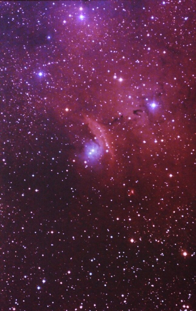
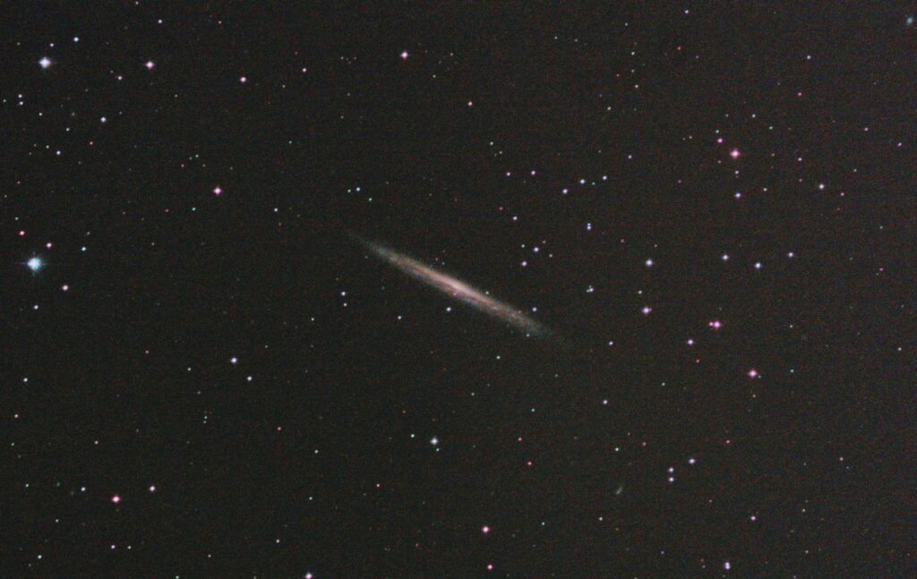
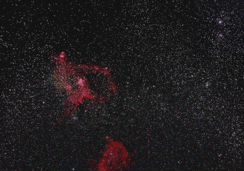
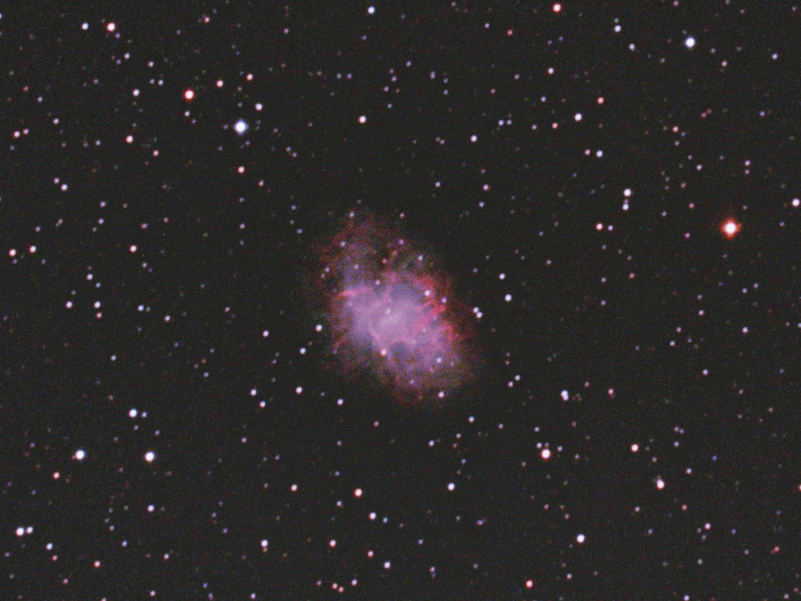
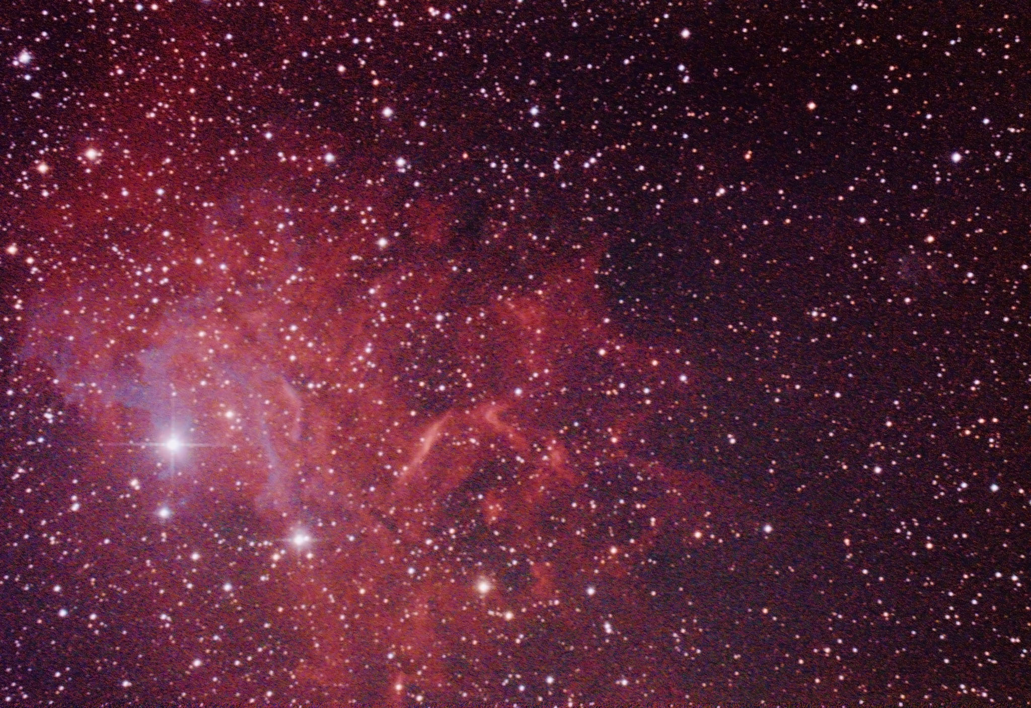
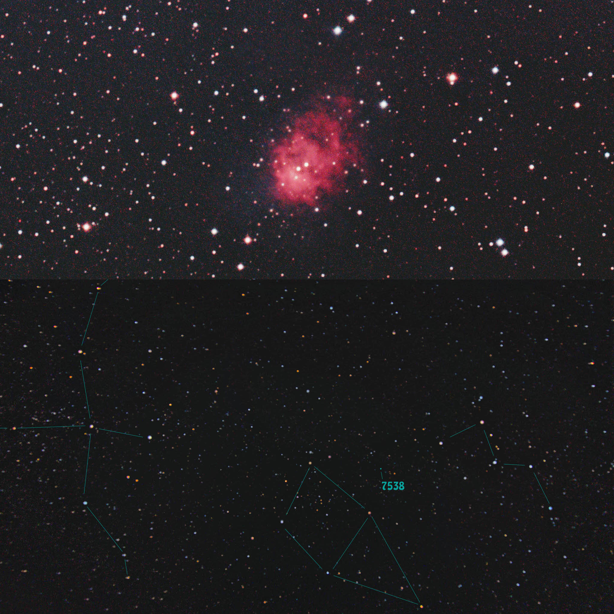
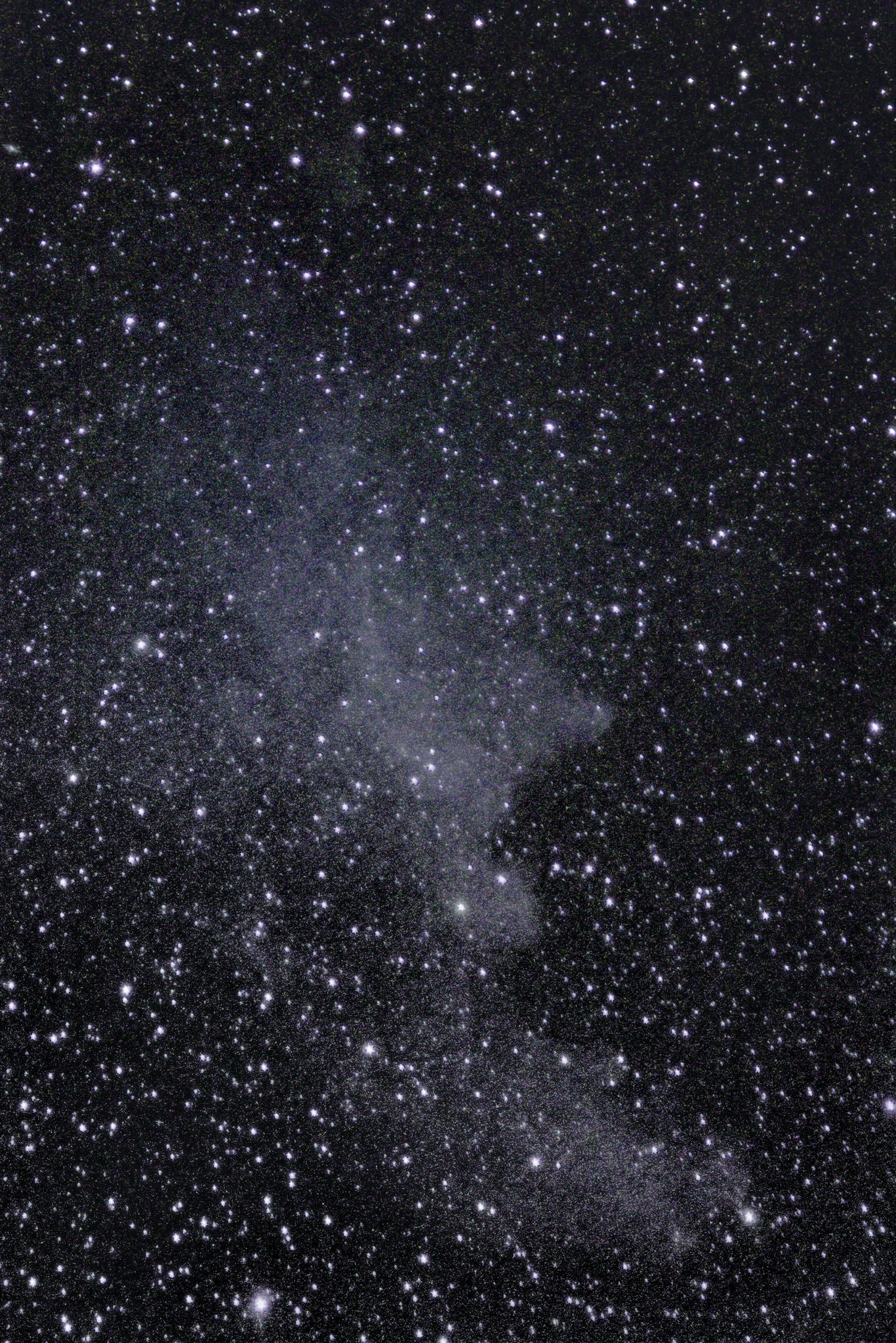
375: IC443 Jellyfish nebula – 2025/3/20
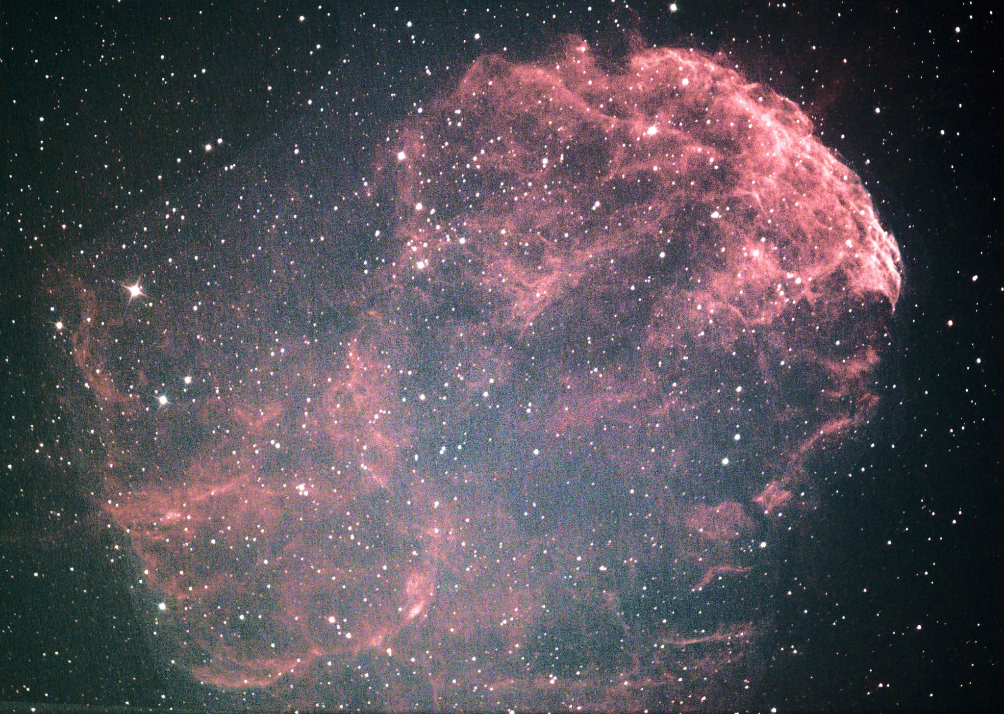
2025/3/20~21 from Sunnyvale California
Newtonian reflector of 250mm diameter with 1000mm focal length on CGEM with Quattro coma corrector, controlled by CPWI without autoguiding,
filtered by Svbony SV220
Lights: 300 x 15 secs, Darks: 30, Flats: 30 were taken with ZWO ASI294MC PRO.
Software:
SharpCap
Gain=420, Exposure=15,
White Bal (B)=95, White Bal (R)=52
Brightness=39, Gamma=94, Temperature=2.5
DSS, Noise Ninja, GraXpert, GradientXTerminator, Photoshop CS5
Year 2024~25
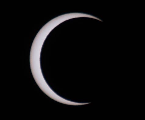
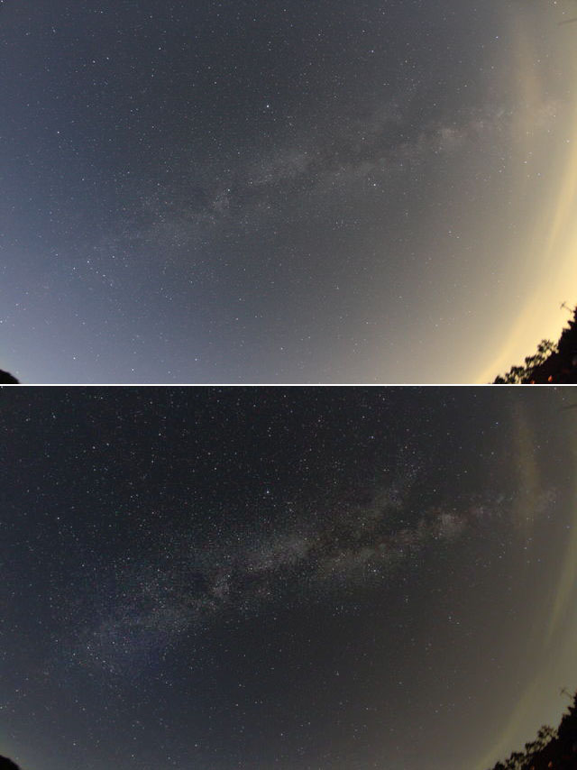
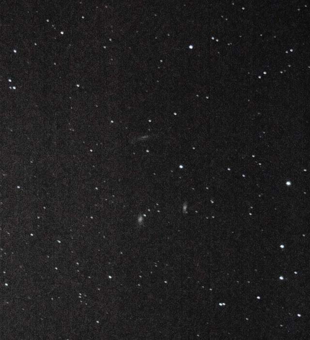
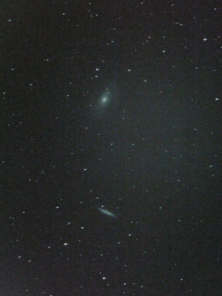
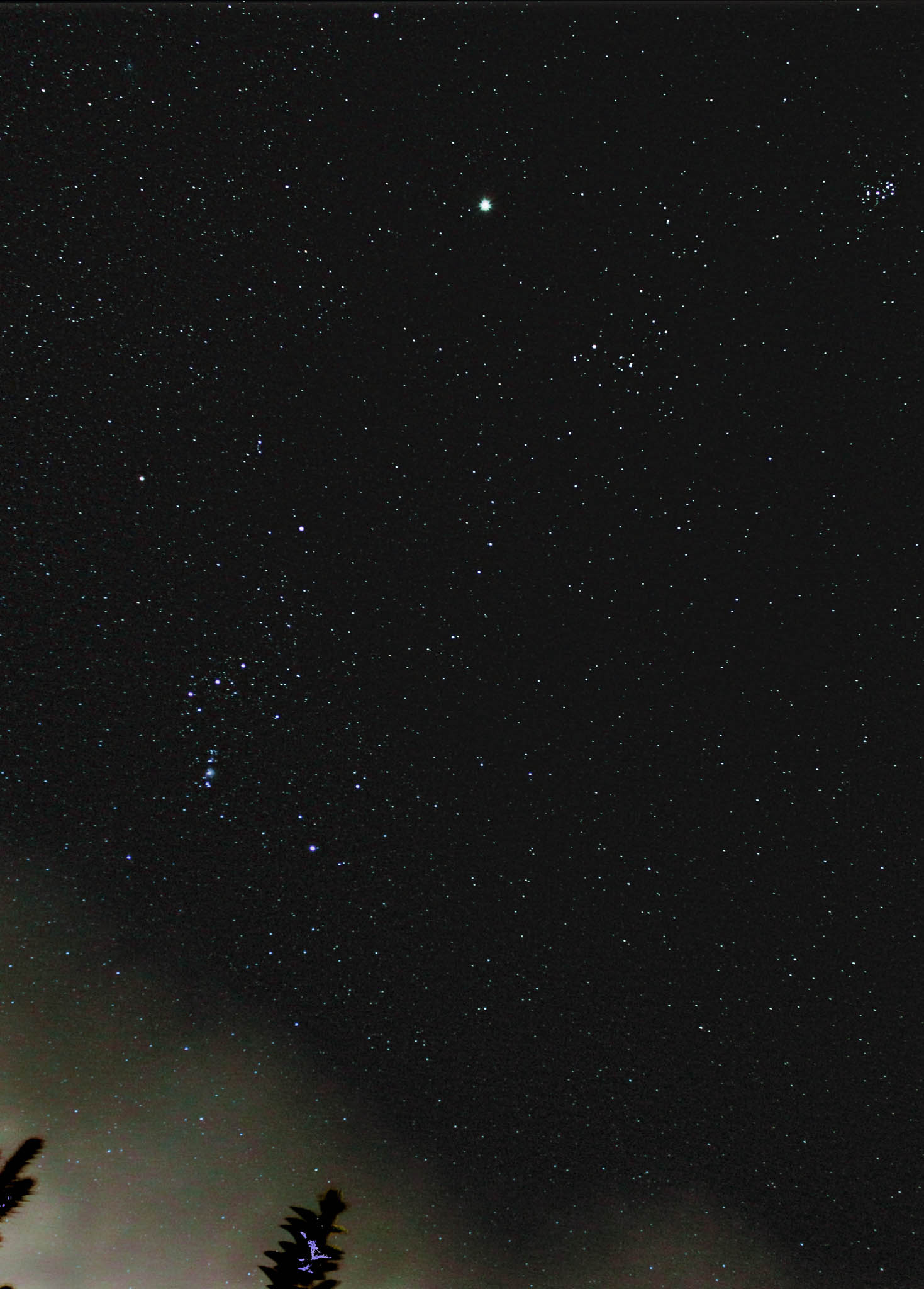
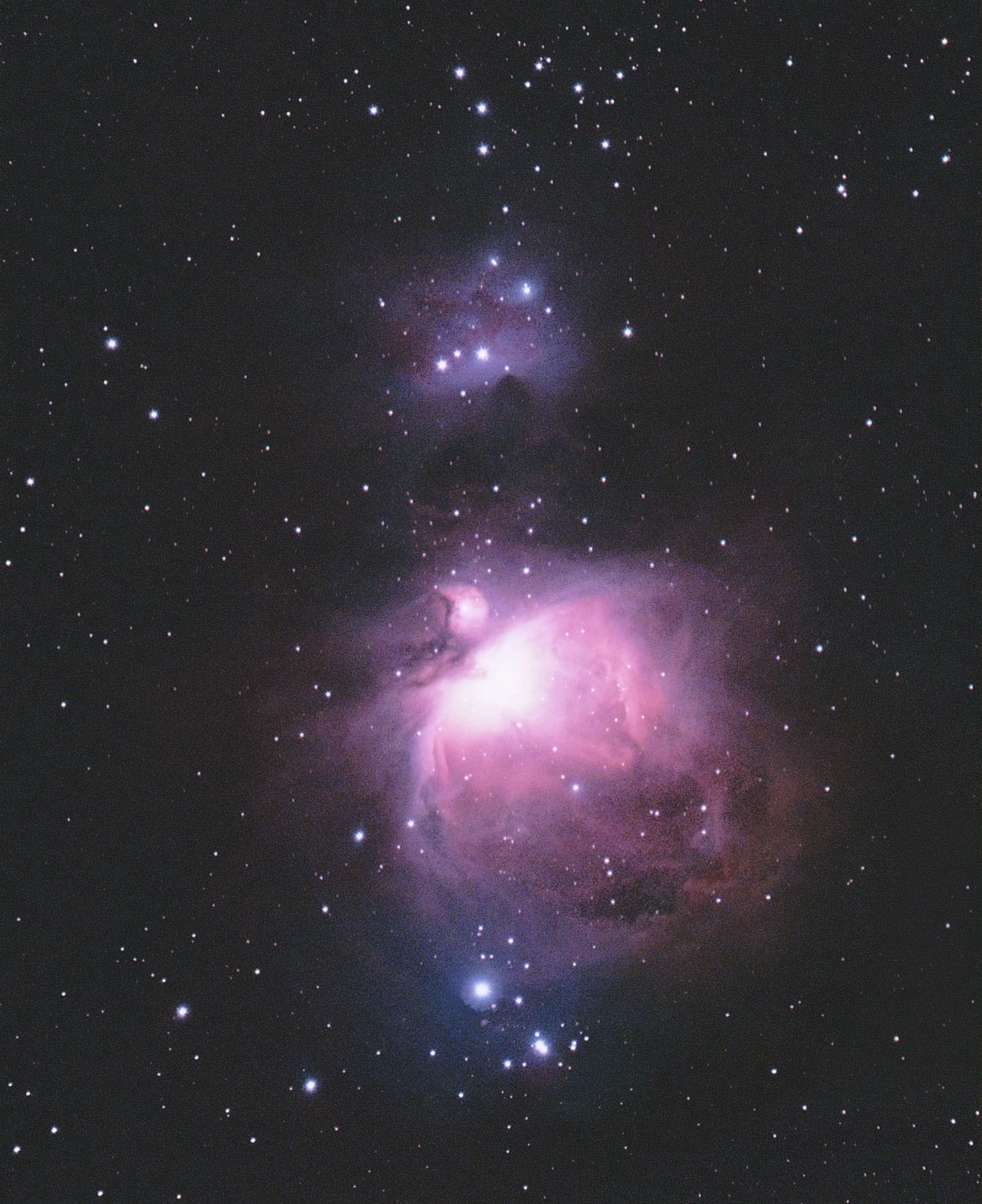
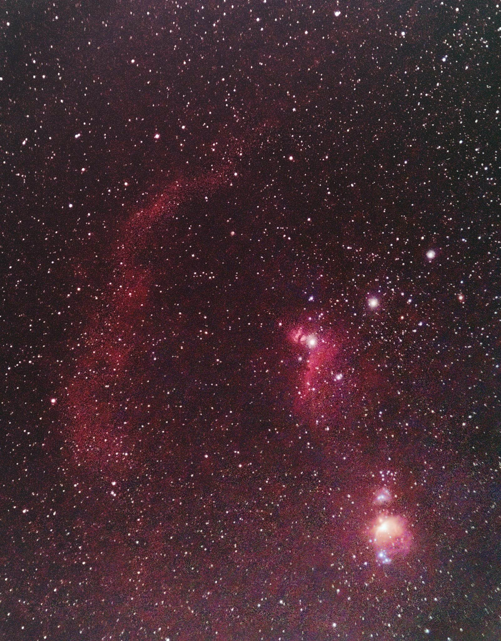
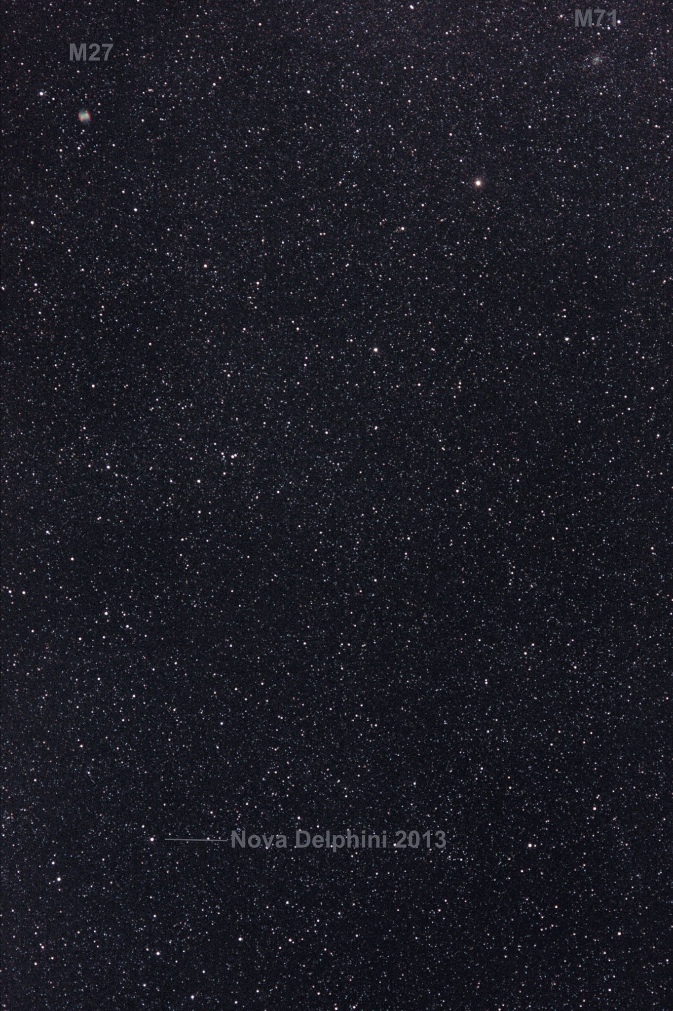
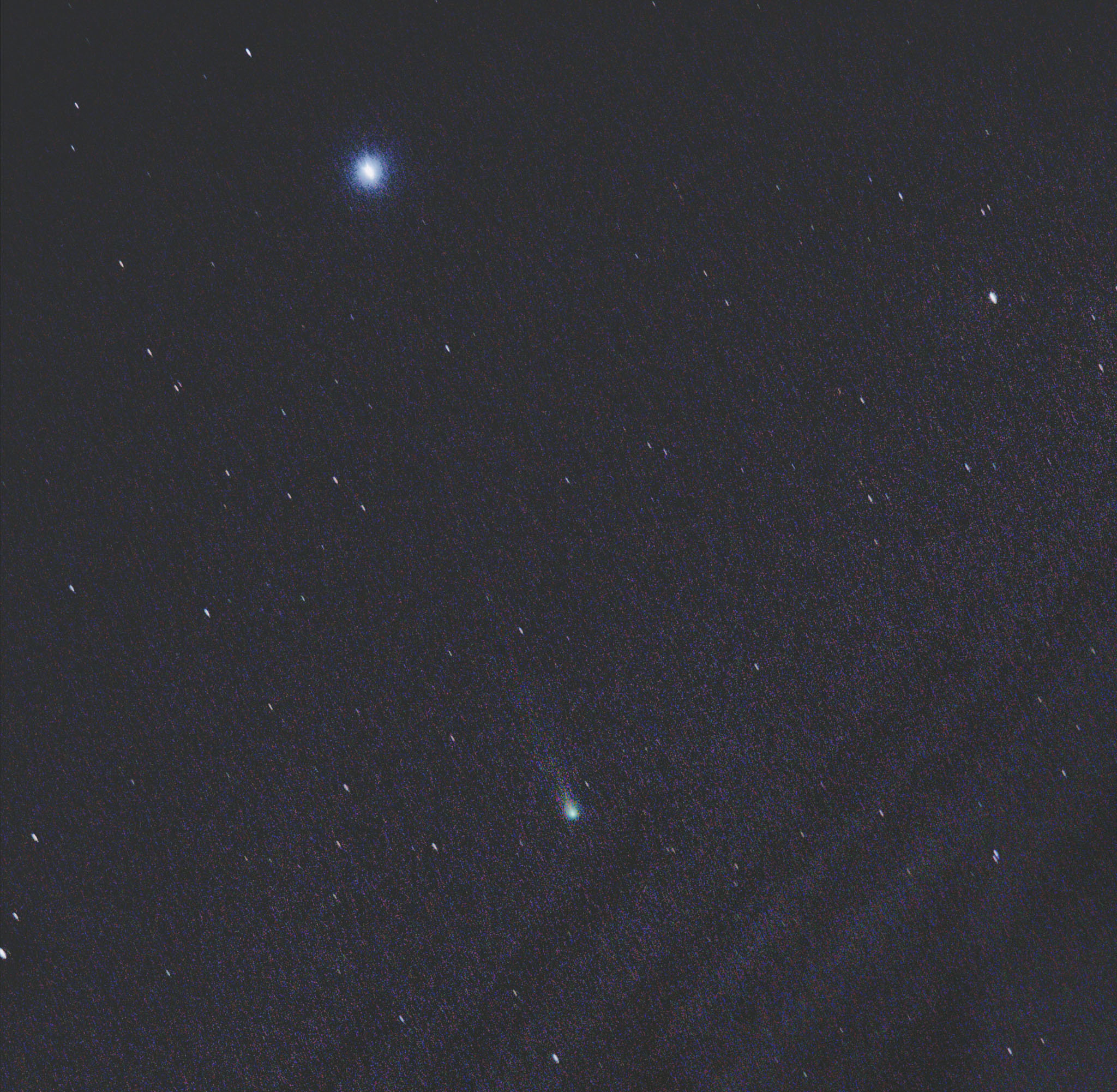
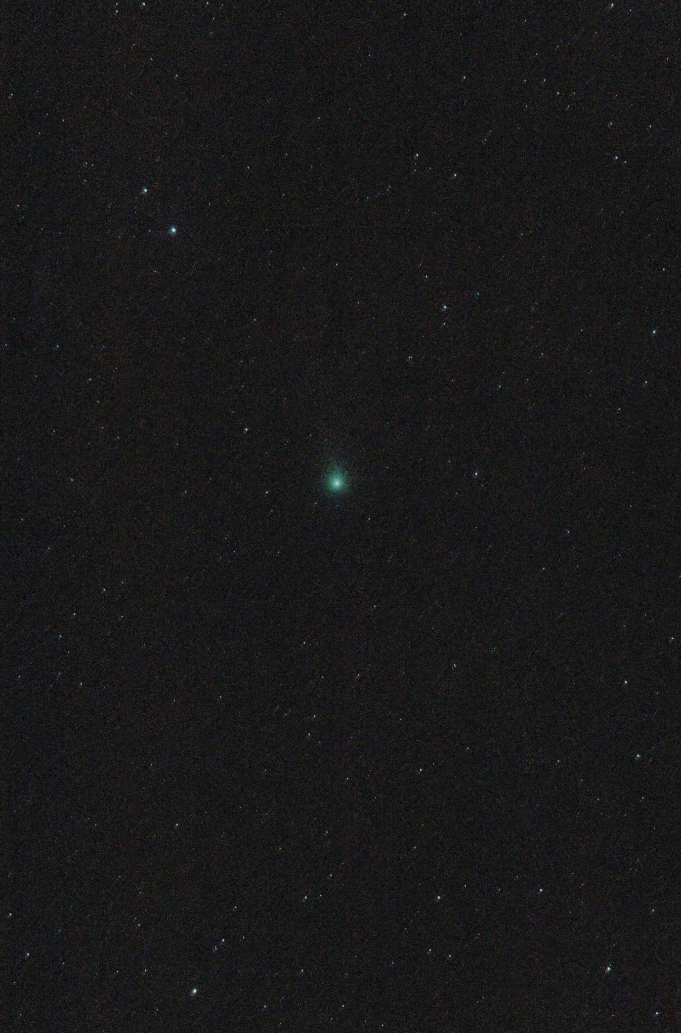
372: Comet C/2023 A3 紫金山ーアトラス彗星 – 2024/10/18
9月下旬に地球に接近し、現在(10/18日)太陽から離れつつある、彗星C/2023 A3 (「紫金山」Tsuchinshan-ATLAS)です。ペアー写真1、10/13 7:30撮影、はSigma 150-500mm@150mm,F5,Canon 6D、でそれぞれ2秒x5フレームをスタック。写真2、10/16 7:40 の撮影、はEF 24-105㎜@100mm F4.0 L レンズで、カメラは同じ。2秒x243フレームで多数枚スタック。写真2では、フラットが使い物にならず、XTerminaterの疑似フラット使用。さらにPhotoshopのマスク(忘れてしまっておぼつかない)で輝度・彩度調整。マウントはSirius EQ-G。光害の甚だしい、自宅Sunnyvale、シリコンバレー、からの撮影。
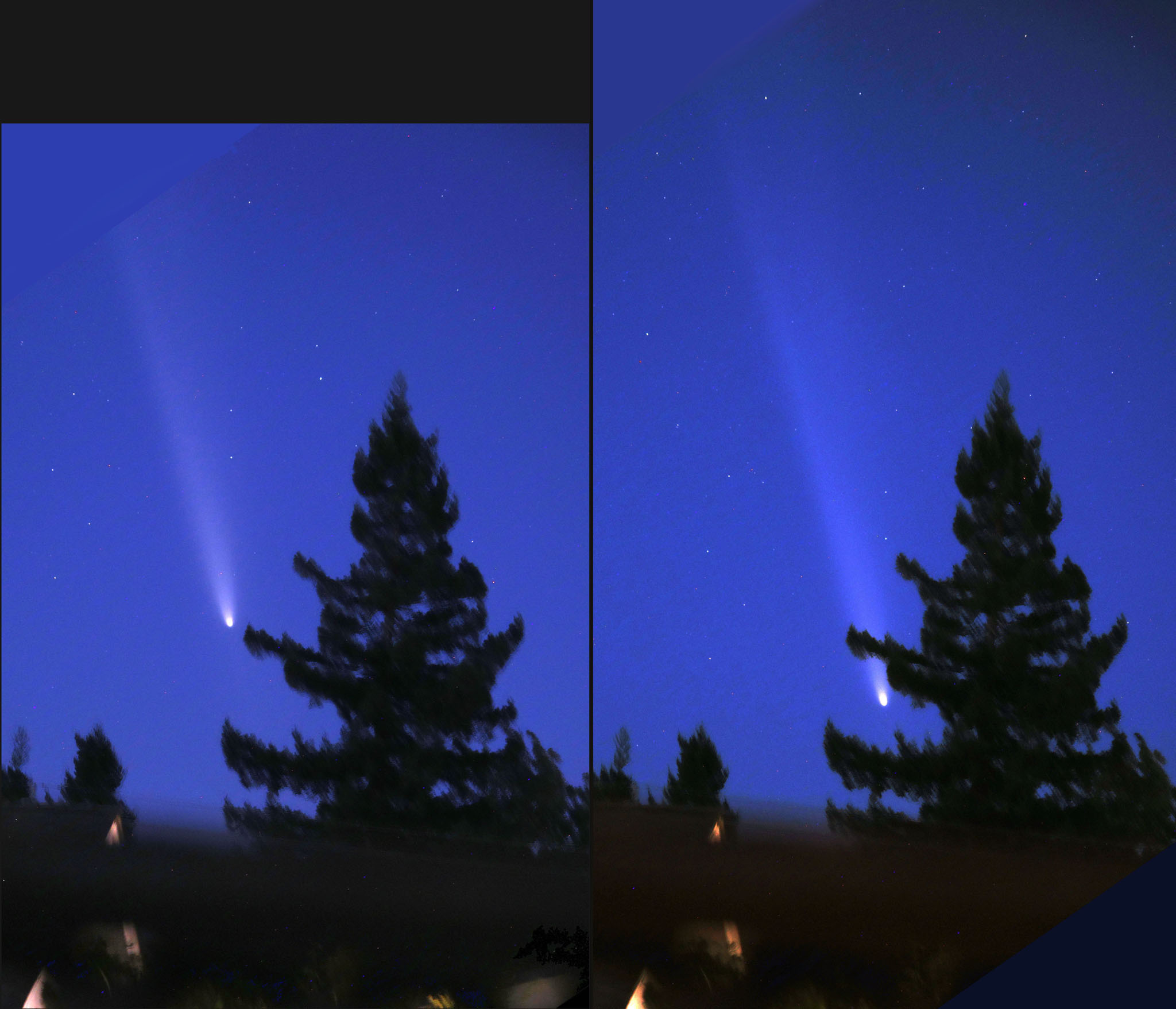
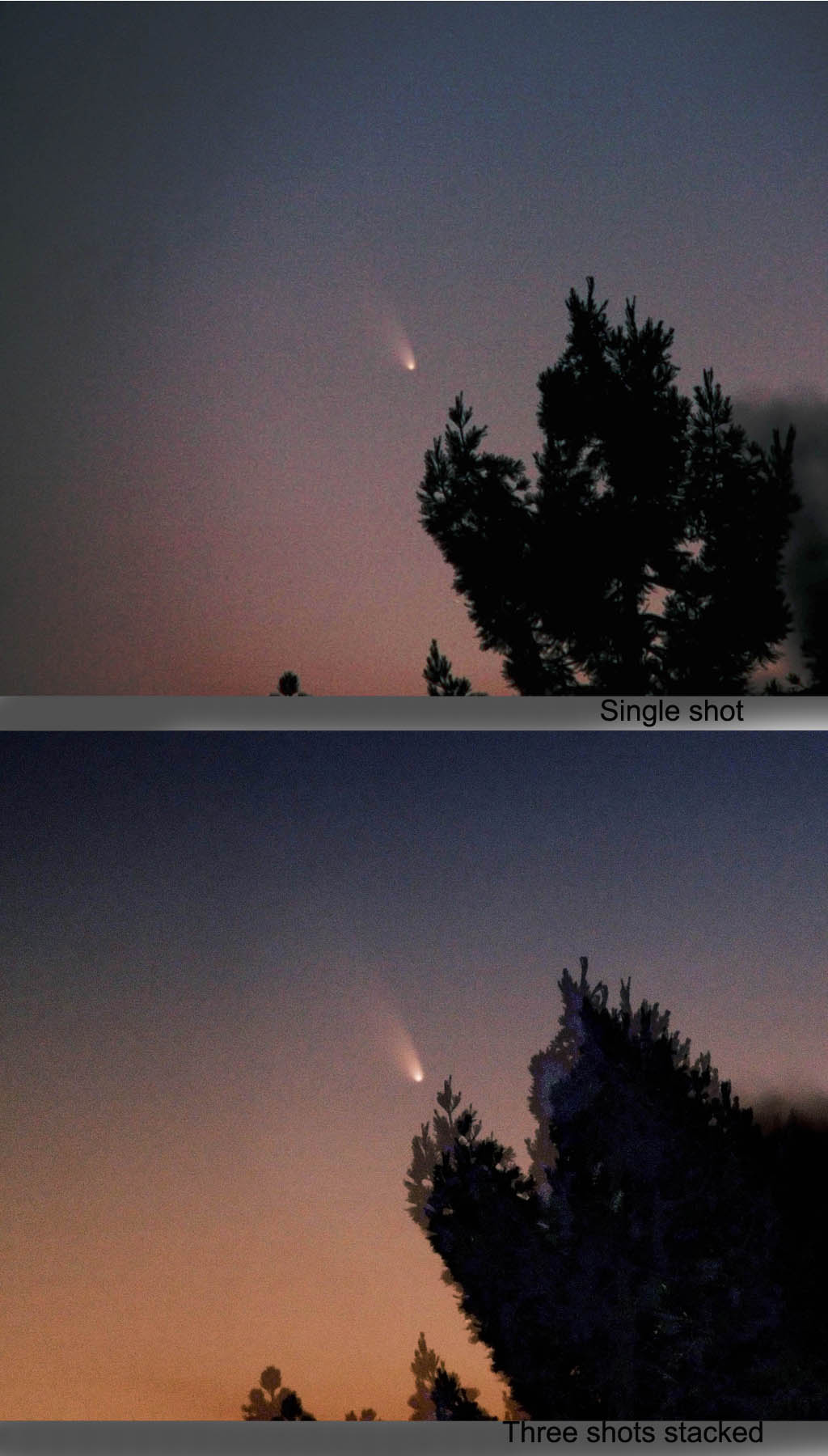
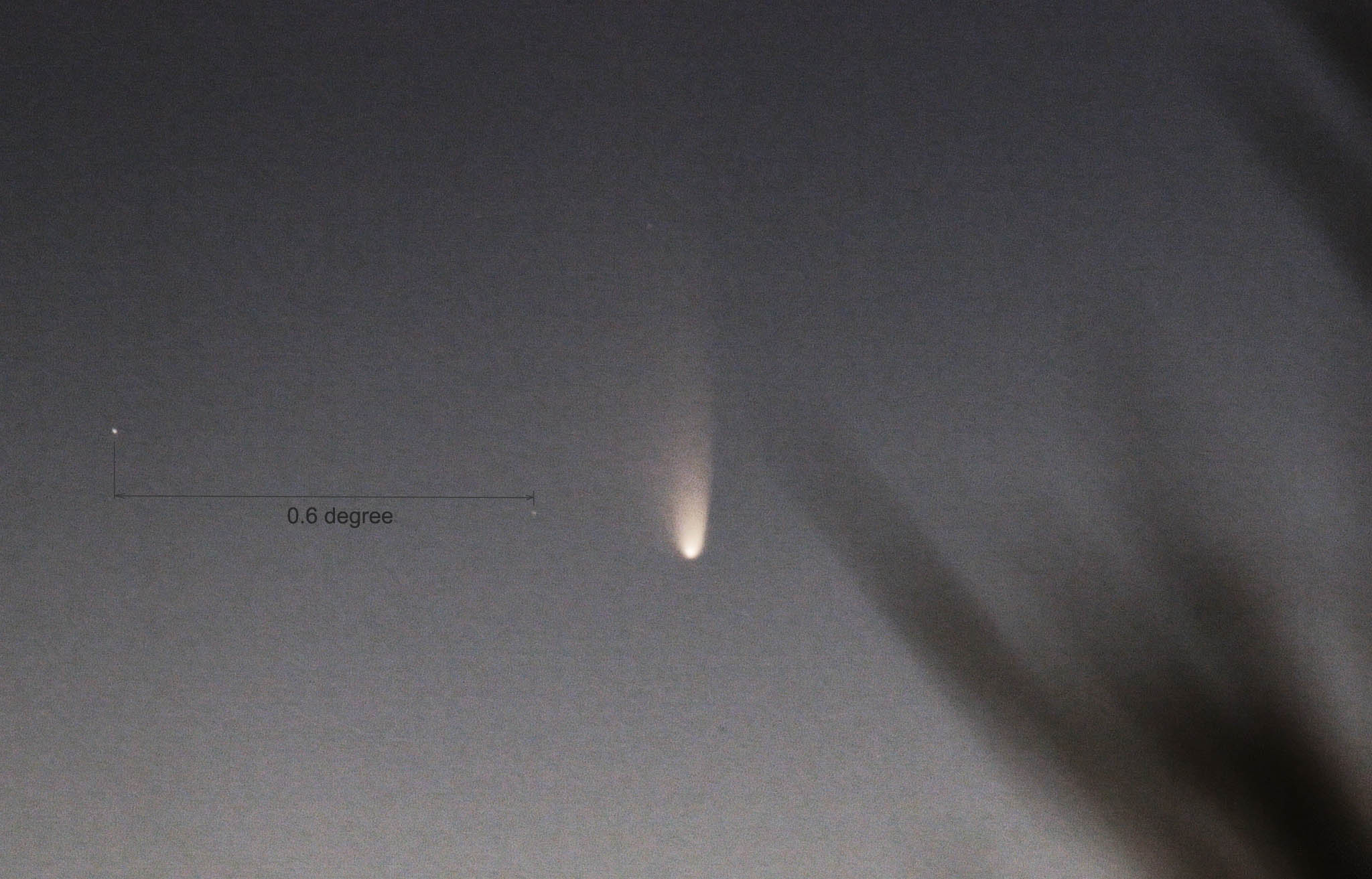
実は10/2に往復200km、サンルイス貯水池へドライブを敢行したんですが、見事失敗。High Way152のVista Pointが真っ暗で行き過ぎてしまい33号線からHigh Way5を望んで「時遅し」の撮影でした(写真3)。満を持した10日後、10/12にはほとんど尾が見えない核のみの撮影で情けない状態でした。
なお、撮影予定だったカリフォルニアのサンルイス貯水池は巨大な人工湖。予定地は以下参照
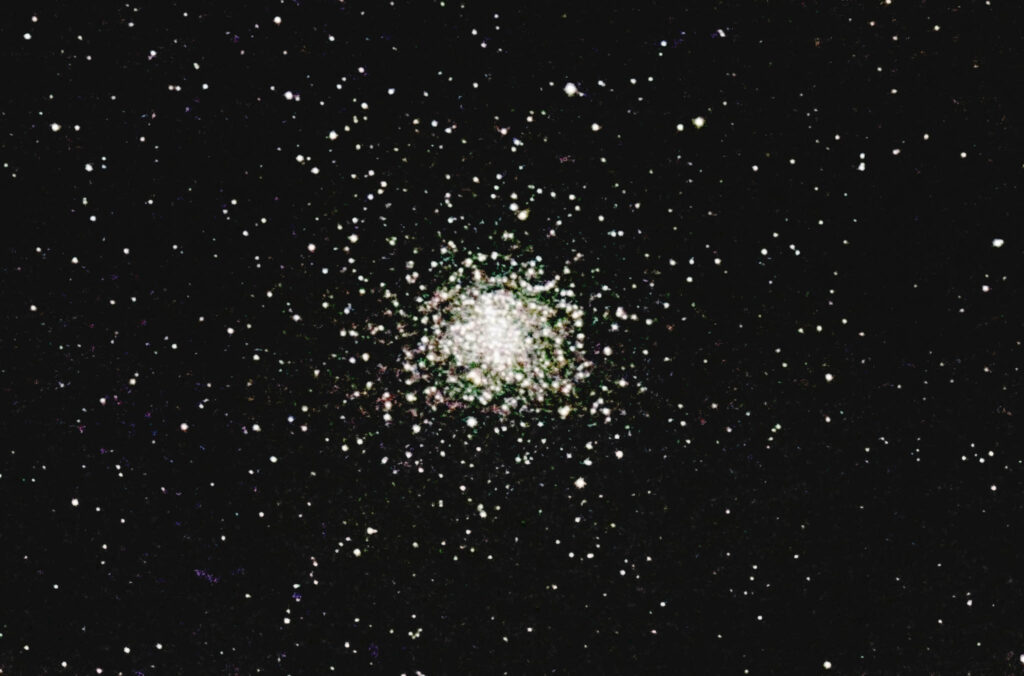
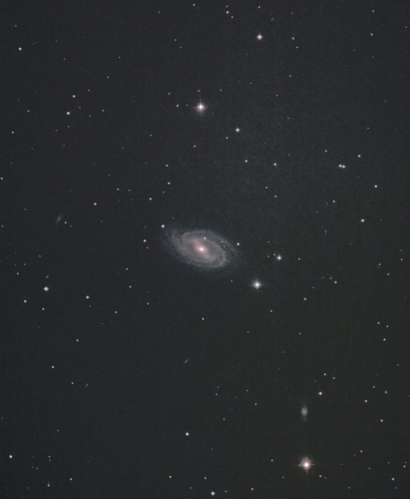
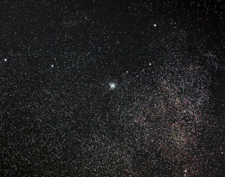
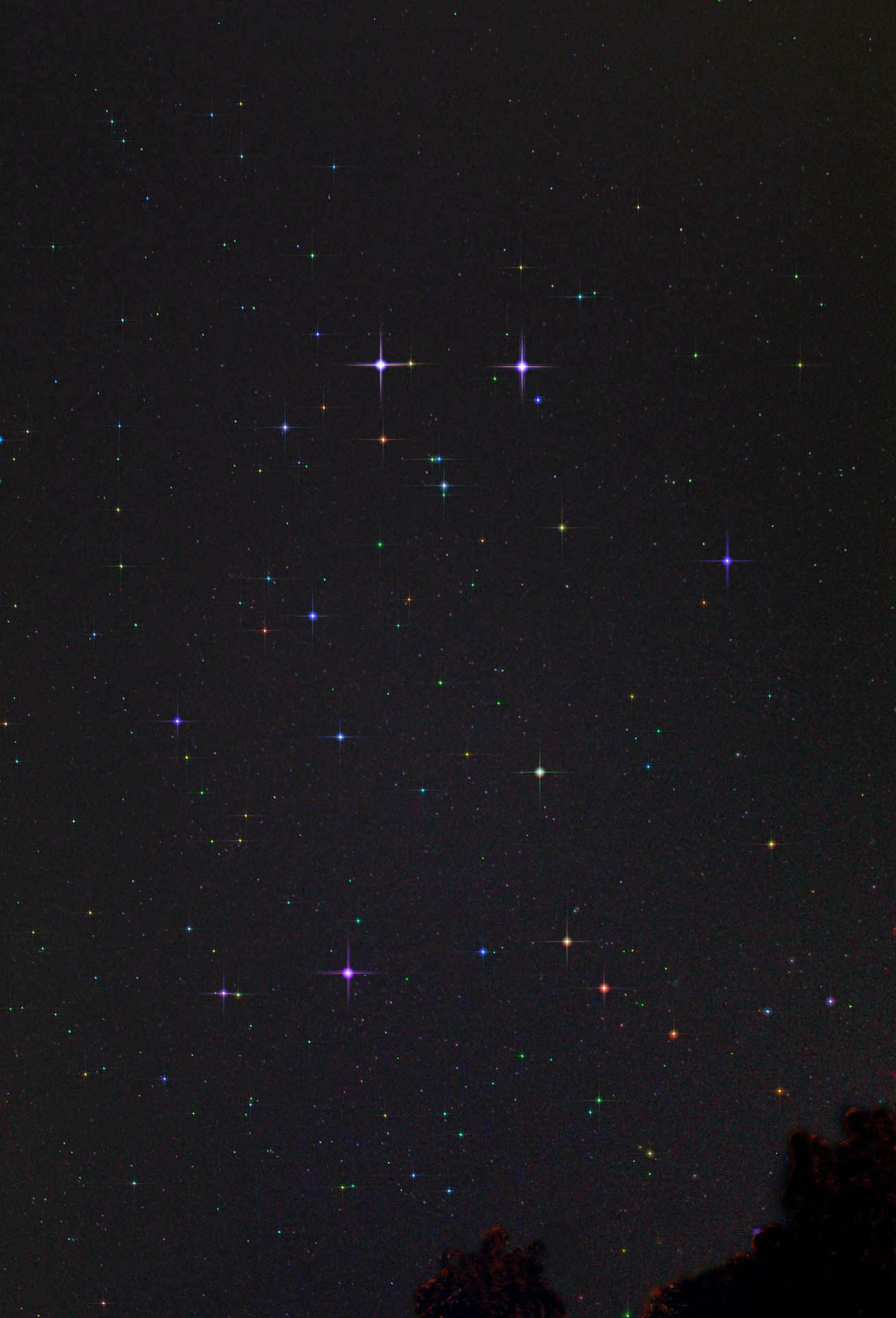
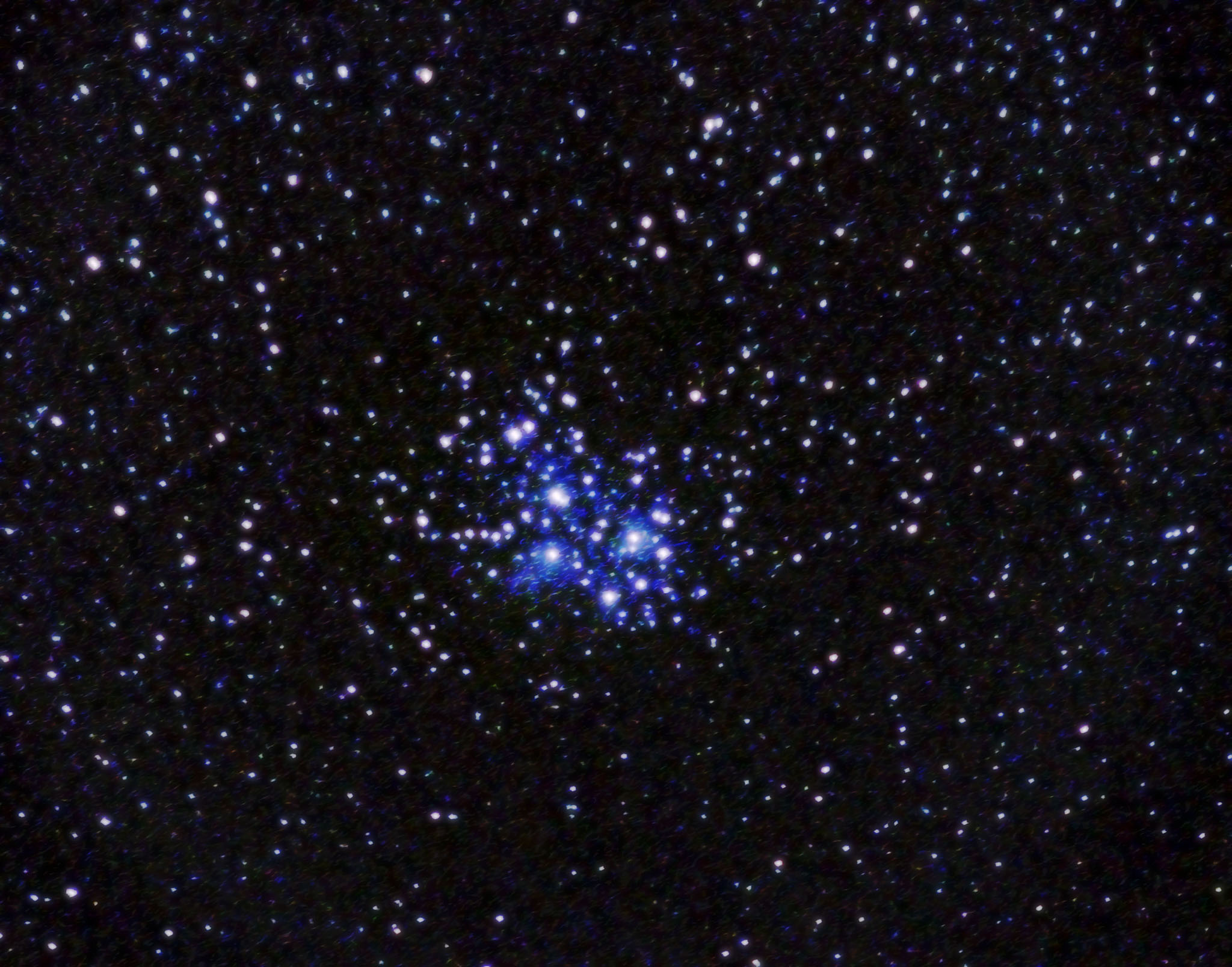
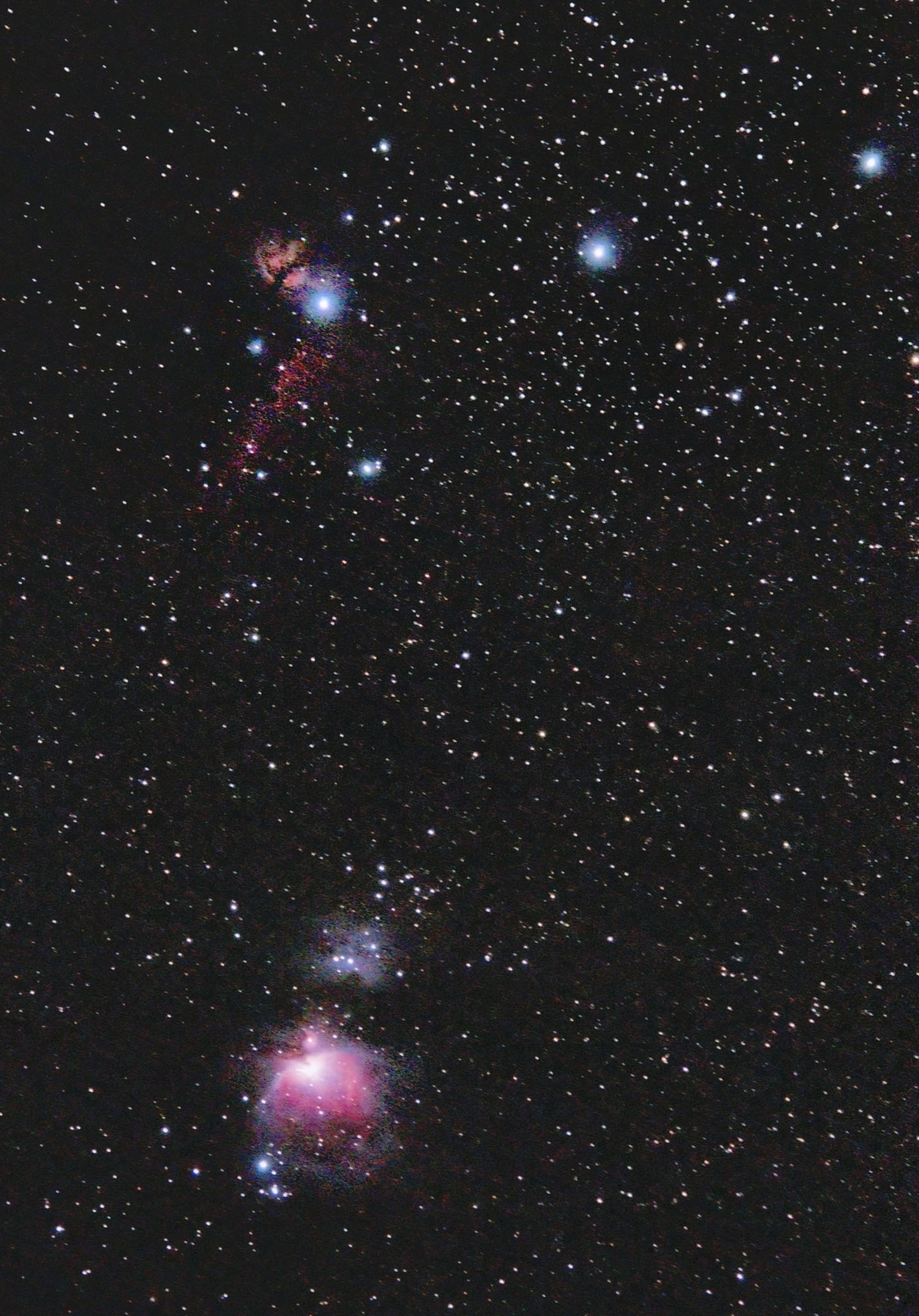
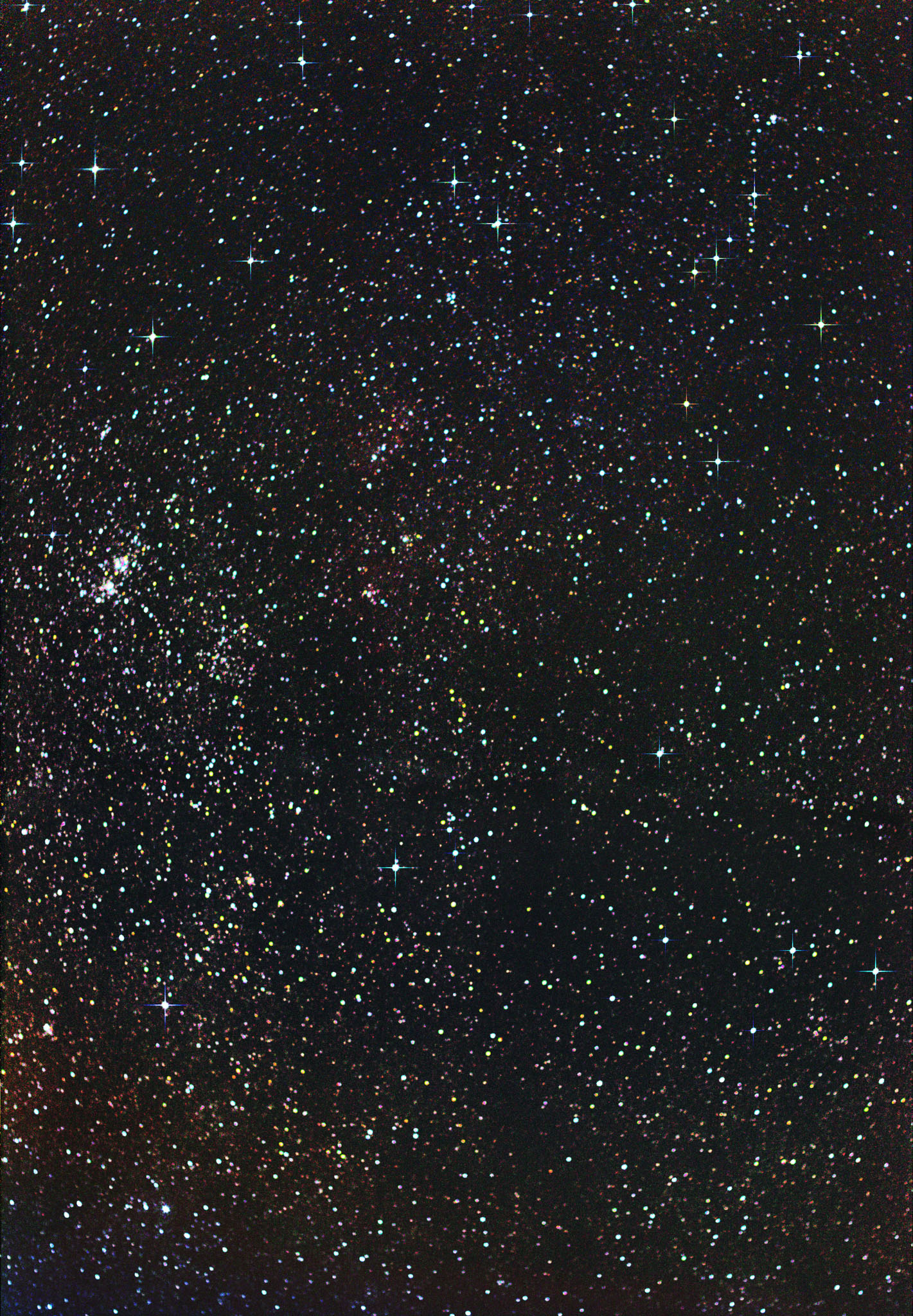
373: M45 (Pleiades, スバル)- 2025/1/5
M45 (Pleiades, スバル)です。望遠鏡は、Skywatcher quattro コマコレクター付きの Orion F4 アストログラフ (25cm DIA および 100cm FL) で、両方とも数年前からリビングルームで眠っていました。

撮影パラメータは次のとおりです。
シリコンバレーのバックヤードから撮影した 2 つの画像のモザイクで、各画像は 15 秒 x 40 コマで撮影されました。20 のダークと 20 のフラット。今回は自動ガイドなし。ガイドカメラ ASI120 と CPWI の組み合わせはUSB接続切れで泣かされます。メインカメラとマウントは ASI294 MC Pro で、3 度 C の温度に設定、CGEM は構造補強しています (Orion F4 は少々重い)。
ソフトウェアは、撮影には Celestron CPWI と Sharpcap、処理には DeepSkyStacker と Photoshop CS5 と Noise Ninja と GradientXTerminator です。PixInsight は、2010 年代後半にはあまり必要ではありませんでした。しかし、そのうち必要になるかもしれません。よろしくお願いします。
Nobuo Urata 2025 年 1 月 7 日
追伸: 100 個以上の天体を含む天体写真を、https://www.alumi-lab.com に移動しました。ご意見ありましたらお願い。(このサイトは安全だと思いますが、Chrome でときどき警告が表示されます)。
以前は、出来不出来を気にせずにできるだけ多くの天体に遭遇することがモットーでした。昨年、モットーを変更。遠くの天体を撮影するのが難しくなってきています。
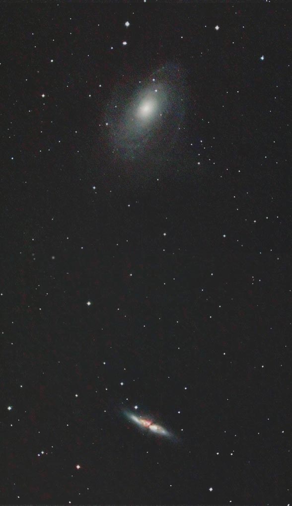
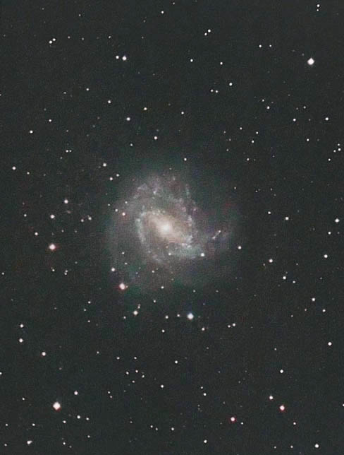
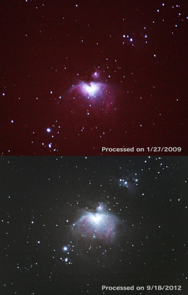
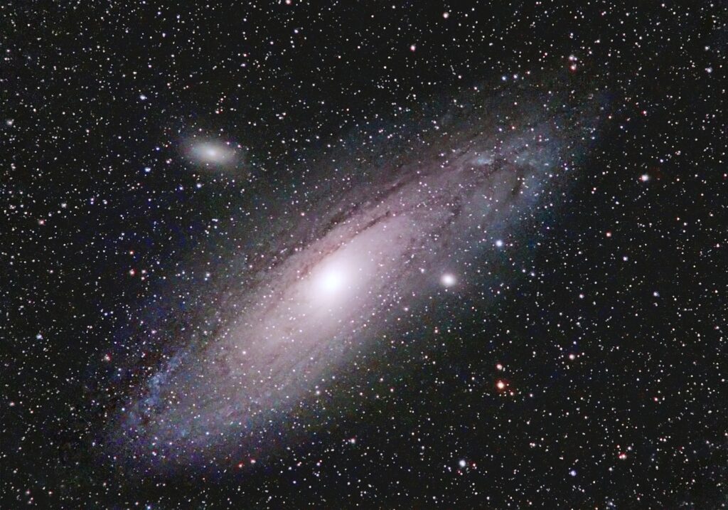
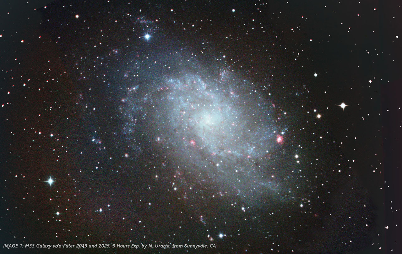
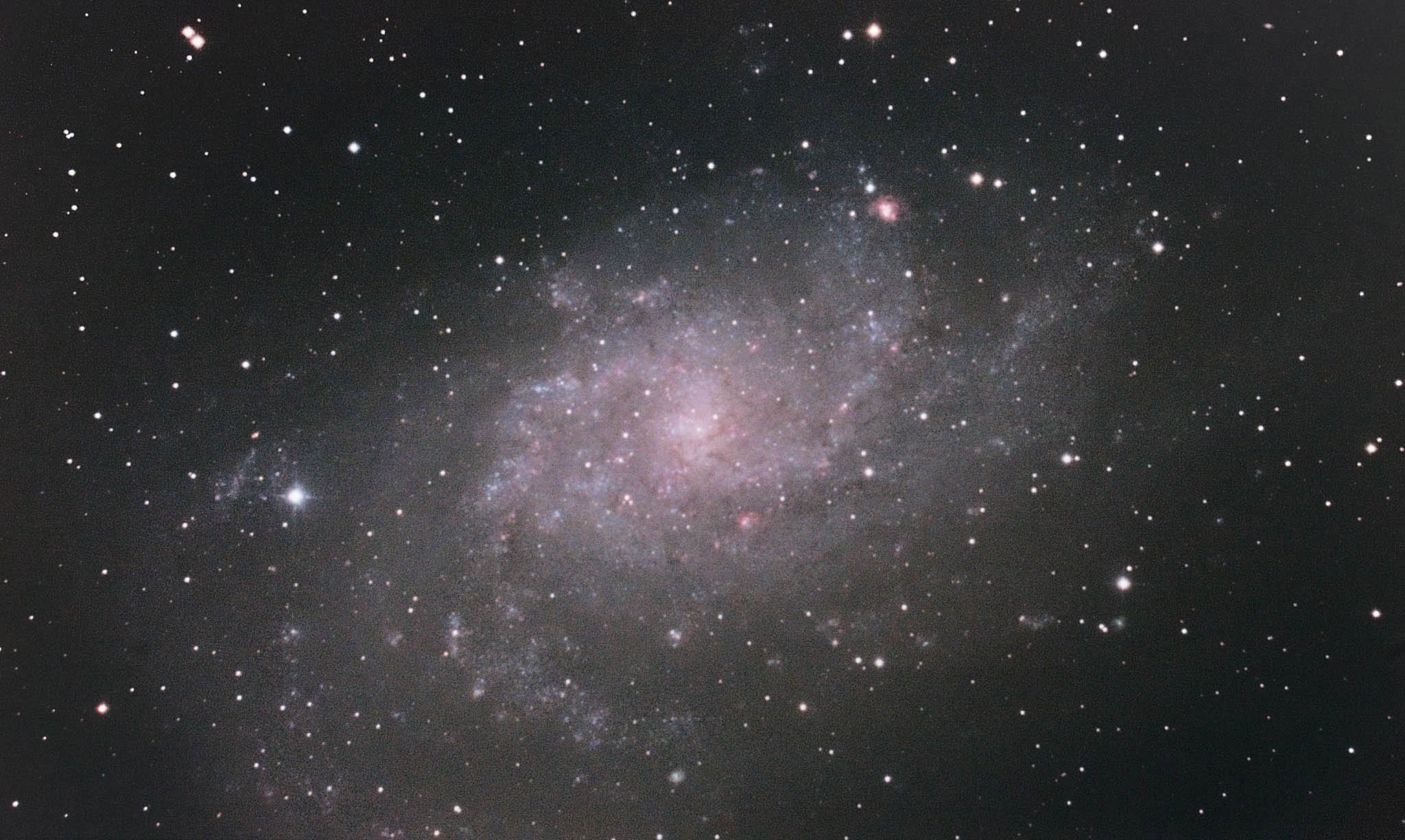
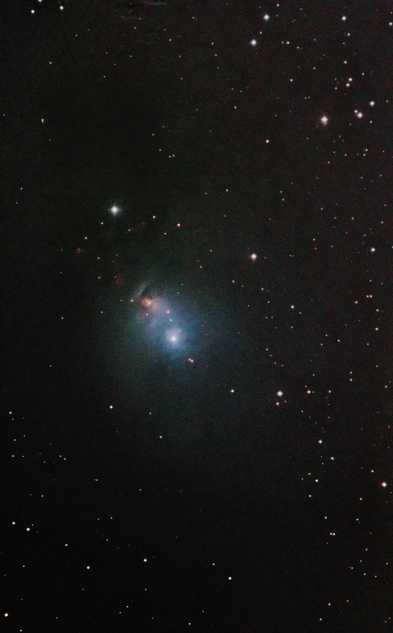
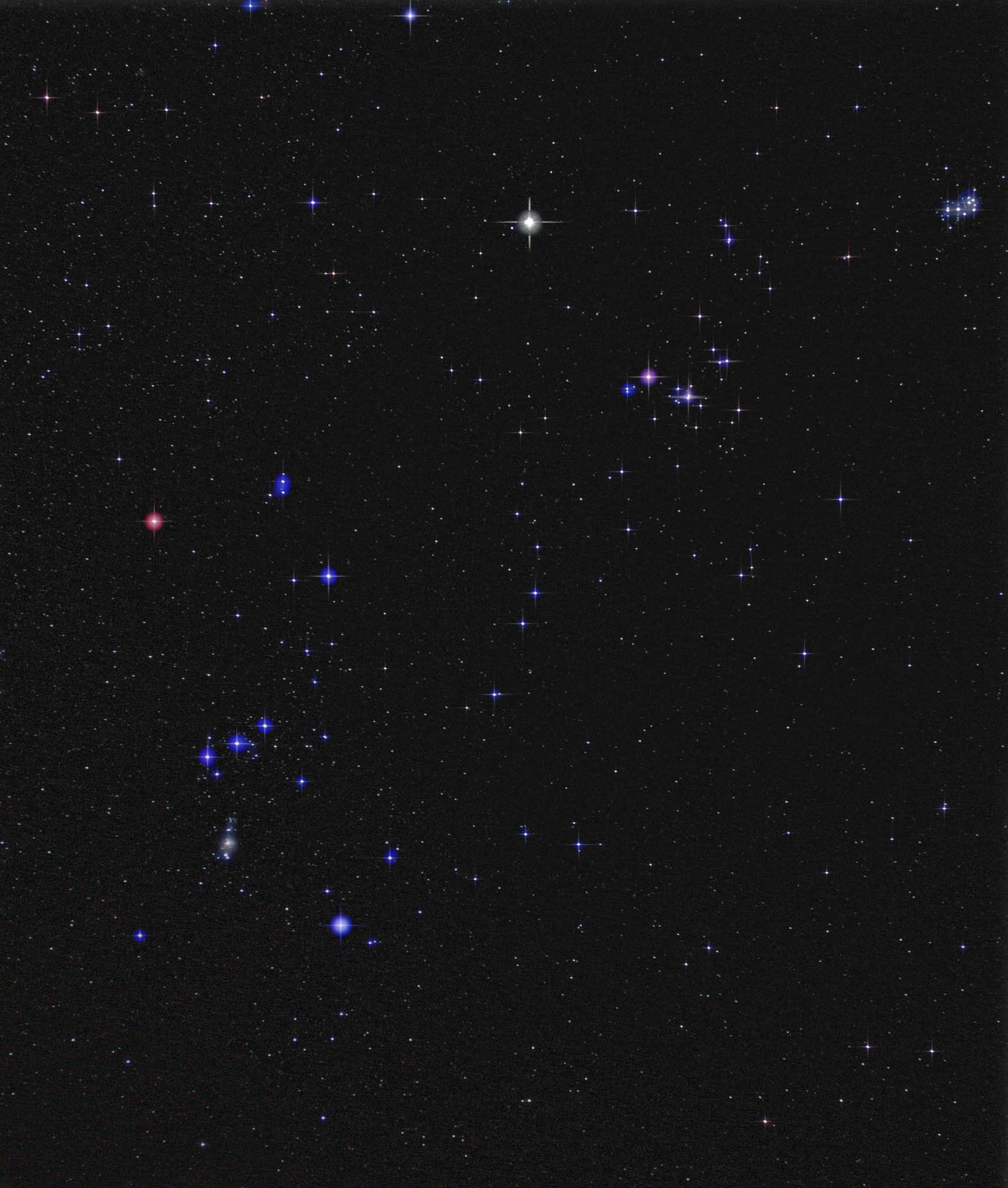
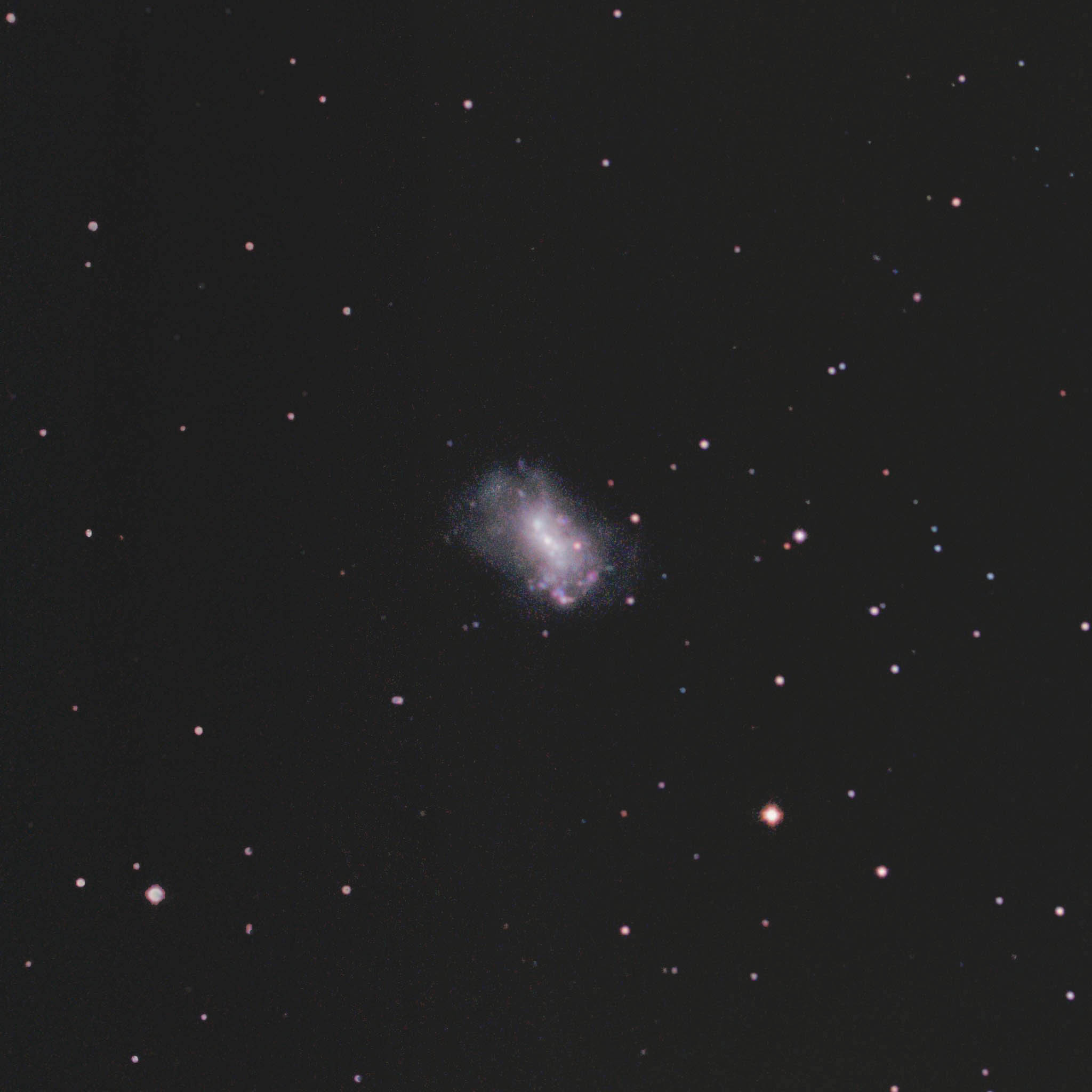
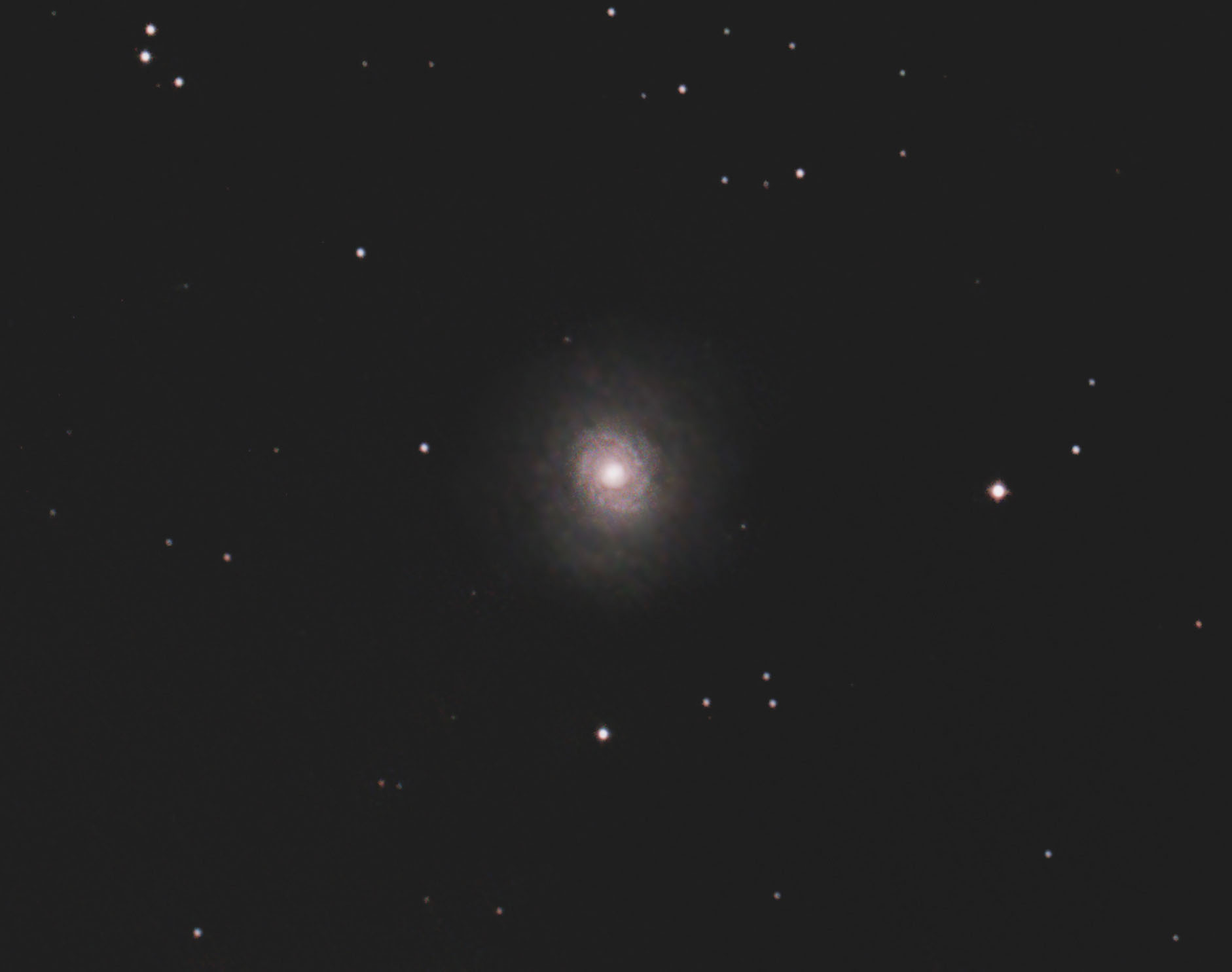
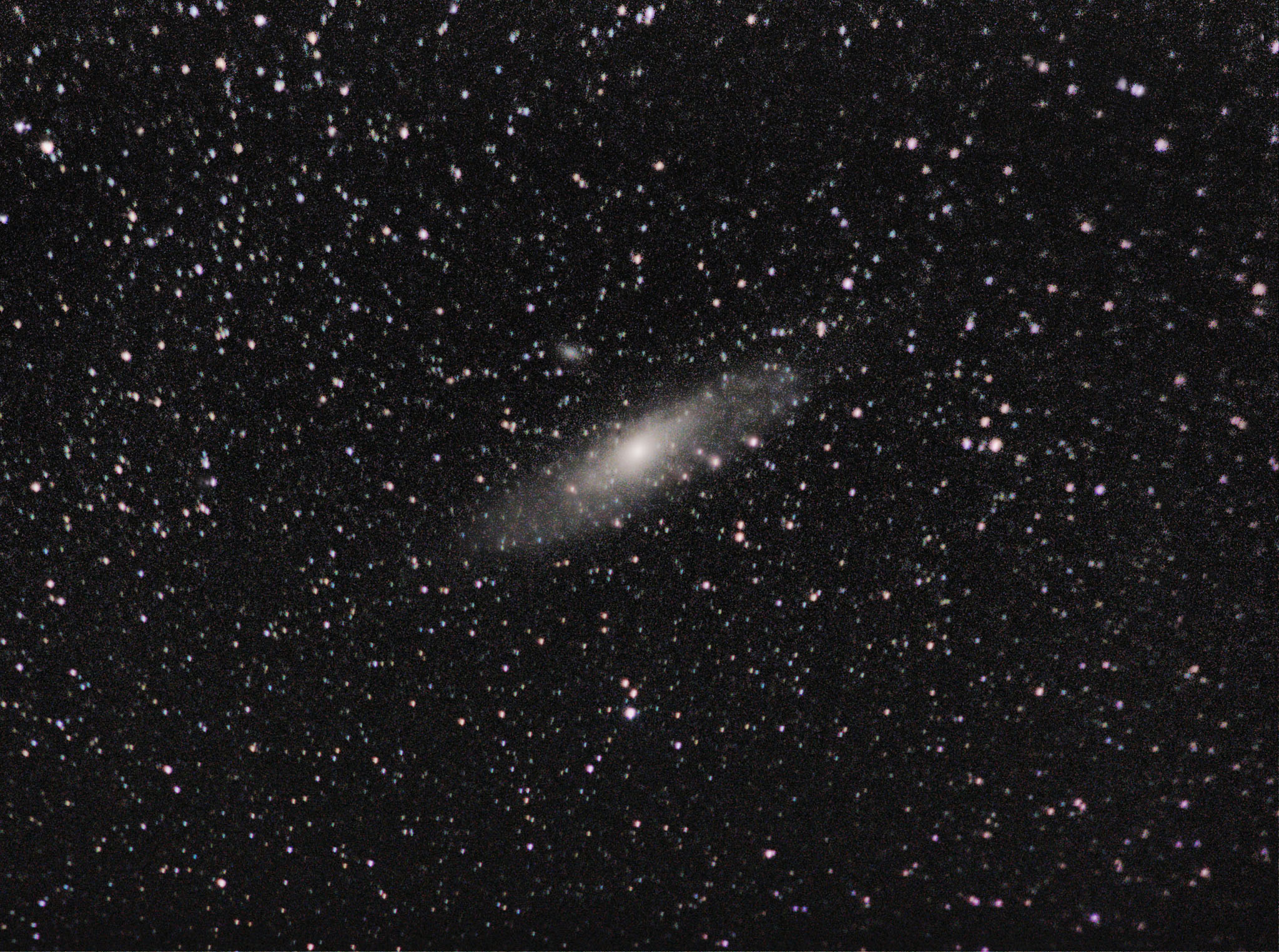
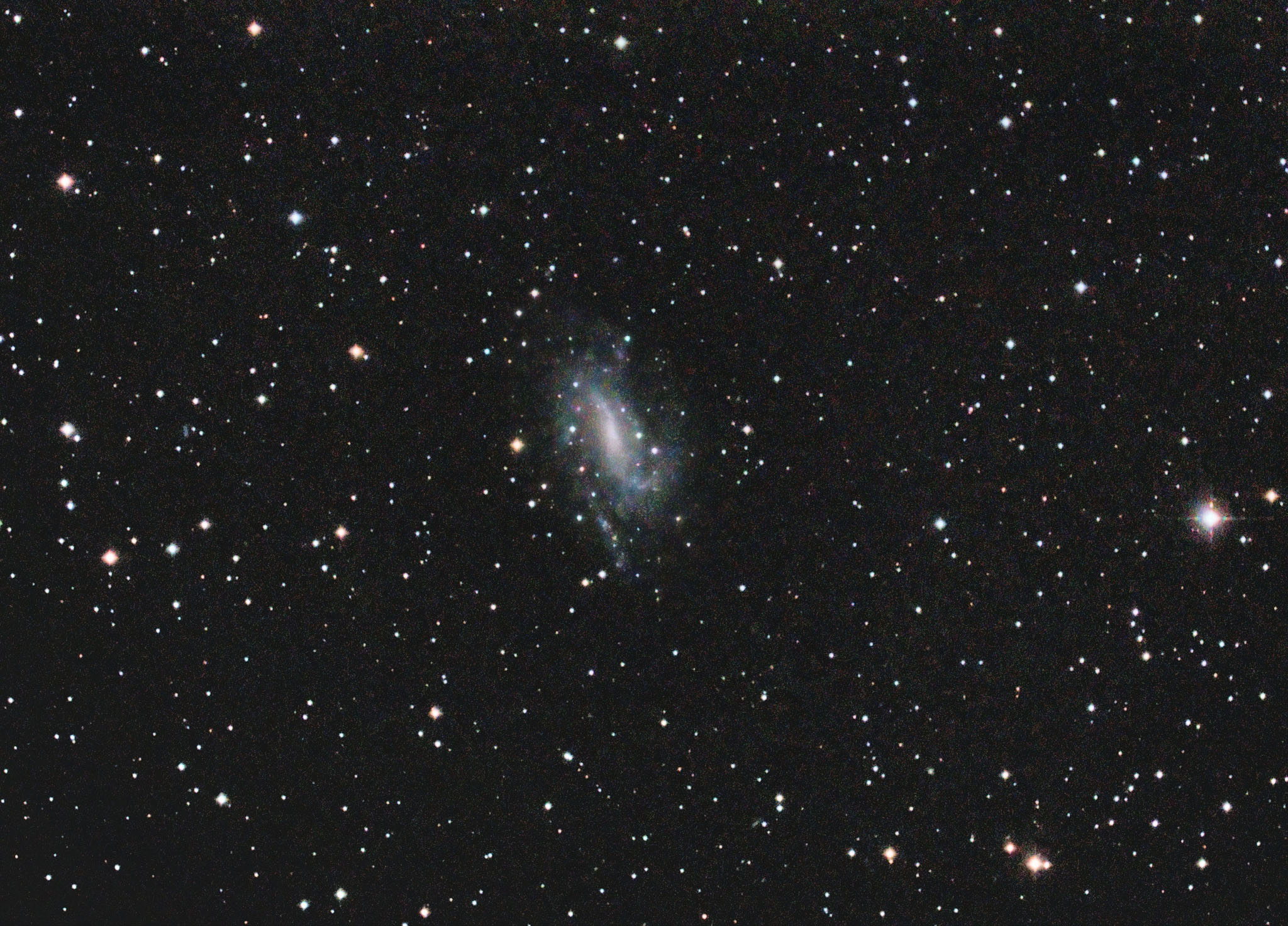
374:M33 w/wo Dual Band Filter – 2025/1/23
IMAGE 1:2025年1月23日にZWO ASI294 MC ProとF4 10インチニュートン望遠鏡を使用して撮影。この画像は、2013年にVIXEN VC200L /F6.4とEOS Rebel XSIを使用して撮影された別の画像と合成されてます。合計露出時間は約3時間です。シリコンバレーの光害にもかかわらず、M33の渦巻き状の青磁色(青緑)が写りました。
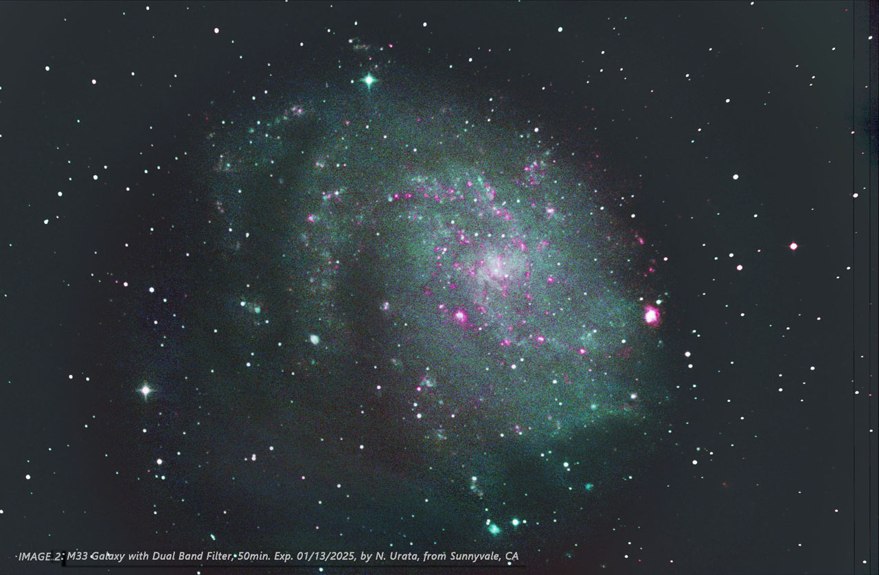
IMAGE 2:SVBONY SV220、デュアルバンド(H-アルファとO-III)フィルターを使用しました。満月の空で(2025年1月13日)使用されています。ちょっと驚きは、M33の外側の渦巻きが、わずか50分の露出時間で出たことです。
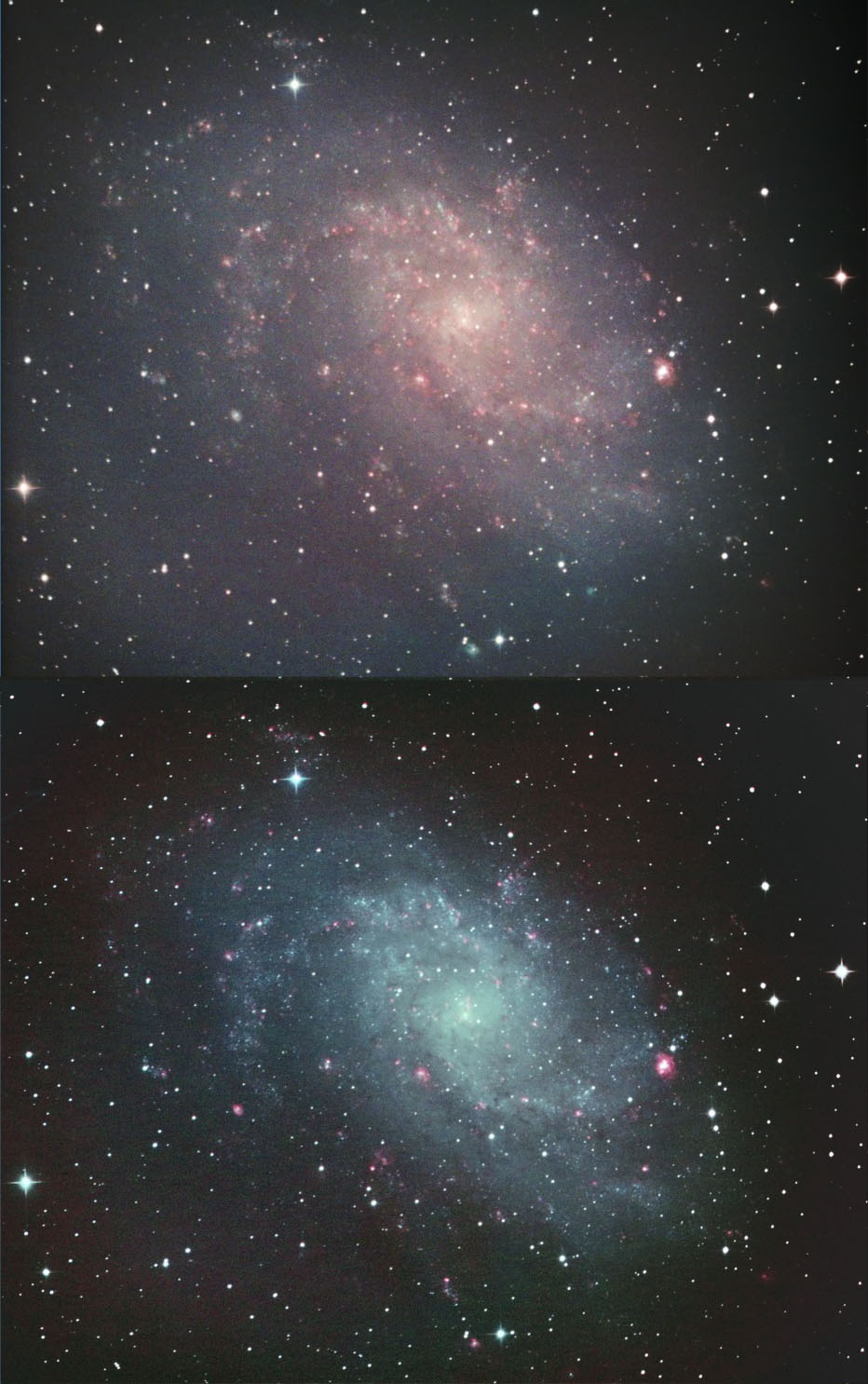
最後に、二画像(H&OとRGB)を異なる重みで合成しました。2つの合成結果、画像3と4を添付しました。
IMAGE 3: H(50%)、R(50%)、G(100%)、B(100%) – R の半分を H の半分で置き換え。
IMAGE 4: H(100%) がをR にライトニング (Photoshop) -たぶん加算処理。さらに、背景を GraXpert 3.02 でフラット化すると、赤みがかった背景がニュートラルに、同時に、白っぽい渦巻きが青に変わります。これは補色変化を使用する手法です。 この色合いが気に入っています。
コメントをお待ちしています。とくに 「O」の使い方は? また、O-III 放射の物理、またそれがどこから来るのかを理解してません。
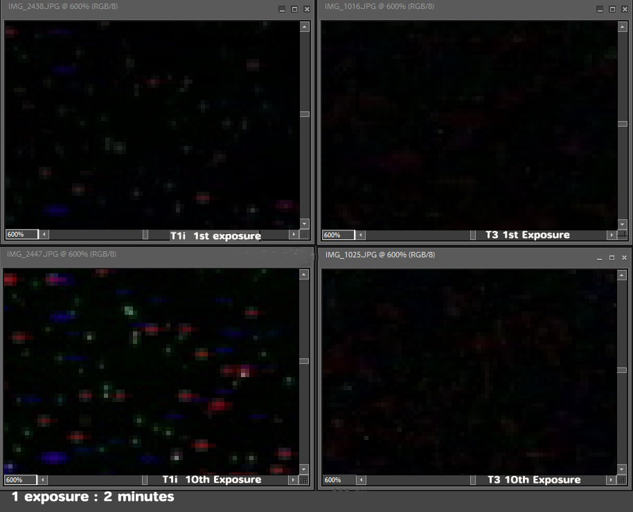
粗い写真、不完全な星の形や色で申し訳ありません。露出時間は、ASI294 では 15 秒/コマ、EOS では PHD ガイドで 3~5 分/コマです
浦田
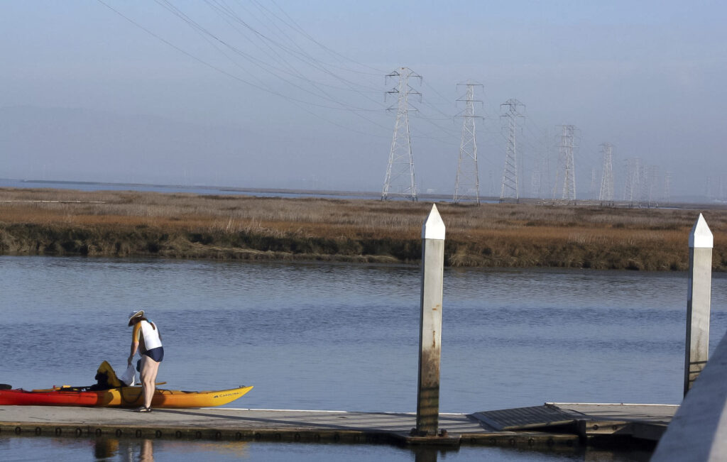
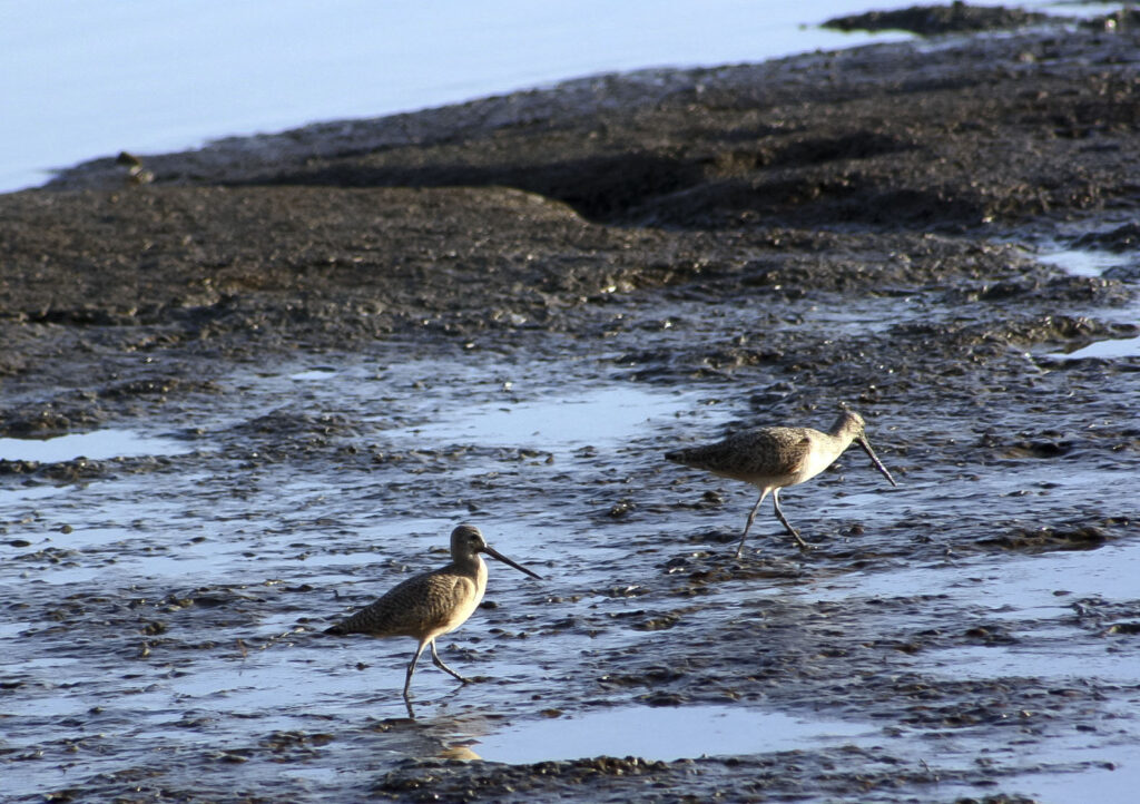
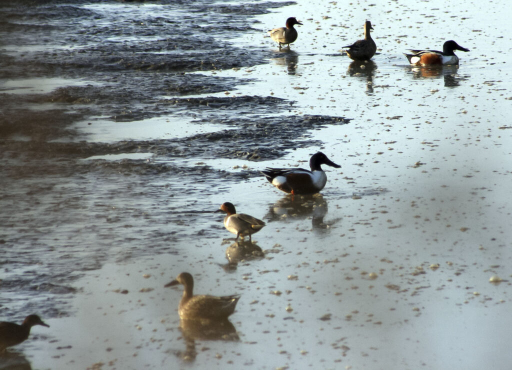
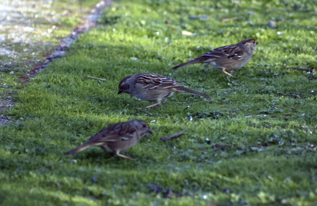
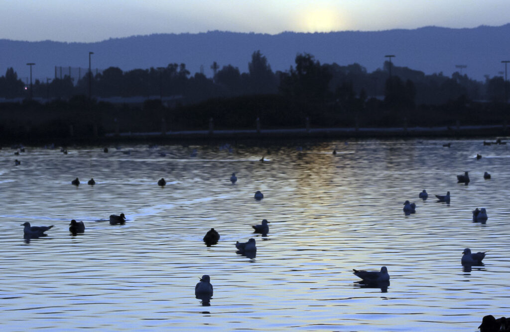
Bayland in Palo Alto CA


Year 2013


Year 2012